Language is used across all known human populations, but the languages used across these populations also exhibit striking differences. A longstanding goal in Linguistics has thus been to identify universal features of language: characteristics that are shared across all human languages. Understanding which features appear to be invariant across languages would shed light on the origins of language, as well as the potential biological constraints that act as “filters” for the kinds of forms that languages can take.

A recent paper (Coupé et al, 2019) argued for a kind of quasi-universal features: according to their analysis, languages convey “information” at roughly the same rate of 39 bits per second. This paper has since enjoyed a fair amount of discussion (1, 2, 3). However, I think it’s hard to understand or evaluate this claim without understanding how these variables (e.g., information) were operationalized. Thus, the goal of this post is to briefly describe the analyses performed in the paper.

What is “information”?

The first and primary issue, in my view, is that the term “information” is used rather vaguely in everyday discourse, usually to mean something roughly like “semantic content”. However, “information” also has at least one very technical meaning, coming from the field of information theory; this meaning is both more narrow and in some ways less intuitive than the everyday meaning of “information”, leading to considerable confusion.

Claude Shannon introduced the technical meaning in a 1948 paper called A mathematical theory of communication (Shannon, 1948). Here, Shannon conceptualizes information in the context of communication. A sender is trying to convey some message to a receiver, and sends this message using some sequence of signals. “Information”, then, can be understood in terms of the relationship between each signal produced by the sender and the sender’s intended message: how much does a given signal reduce a sender’s uncertainty about the intended message?

I won’t go into all the details here, but the two most relevant concepts that Shannon introduced in the paper are surprisal and entropy.

It’s worth noting that most operationalizations of these concepts don’t really engage with meaning, i.e., the actual message that the sender is trying to convey. Rather, they’re usually operationalized in terms of the signal system itself–that is, the “information” conveyed by some signal x is not necessarily measured as a function of how much uncertainty X reduces about the space of possible meanings M, but rather as a function of the probability of x relative to the space of possible signals {x, y, z}¹.

Surprisal: more surprising signals convey more “information”

Surprisal is defined as the negative log probability of an event. For example, imagine a “language” L containing four possible “words”: [A, B, C, D]. If all four words are equally likely to occur, then each has a probability of 0.25. Thus, the surprisal of each word is:

-log(.25) ~= 2.

The logarithm of lower probabilities will be more negative than the logarithm of higher probabilities; because surprisal is the negative log probability, this means that lower-probability events will have larger surprisal values. Thus, according to this framework, lower-probability events convey more information.

This may still seem a little unintuitive. What does the probability of an event have to do with how much information it conveys?

Recall that “informativity” here is understood with respect to the reduction of uncertainty. To understand this, let’s contrast a language L1 in which each word is equally probable, i.e., [p(A)=.25, p(B)=.25, p(C)=.25, p(D)=.25], with L2, in which some words are more probable than others: [p(A)=.85, p(B)=.05, p(C)=.05, p(D)=.05]. Now imagine a receiver about to receive signals from either L1 or L2. In the first case, each signal is equally surprising; thus, each signal reduces the receiver’s uncertainty about the impending signal exactly the same amount (approximately 2 bits). But in the second case, some signals are more surprising than others: A is very likely, while the other signals are very unlikely. This means that observing A does less to reduce the receiver’s uncertainty about that signal than observing B. A conveys roughly .23 bits, while B conveys 4.3 bits.

As you can see, the surprisal of a signal, and thus its informativity, is highly dependent upon the underlying probability distribution over signals. This brings us to the next concept: entropy.

Entropy

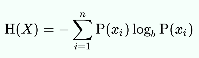
Shannon adapted the concept of entropy from its original meaning in statistical thermodynamics. Shannon entropy can obtained in the following way: for each event i in set of possible events, multiply p(i) * log p(i). Then sum all these products together, and flip the sign. Formally:

Recall that the negative log probability of an event is its surprisal. Shannon entropy takes into consideration the surprisal of all the events in a set of possible events, and provides a measure of–roughly speaking–the expected surprisal value of observing an event sampled from that distribution. Since surprisal is used as a measure of information content, entropy can thus be conceptualized–again, roughly speaking–as the average amount of information produced by some source of events.

This is all very abstract, and using lofty words like “entropy” doesn’t exactly help the matter. Personally, I find that making things more concrete is very helpful.

Consider again two languages L1 and L2. The languages have the same elements [A, B, C, D], but these elements differ in their probabilities. In L1, each word is equally probable, but in L2, the words have the following probability distribution: [p(A)=.85, p(B)=.05, p(C)=.05, p(D)=.05].

Now put yourself in the shoes of a receiver about to hear a signal in either L1 or L2. A receiver listening to L1 has a lot of uncertainty: each word is equally probable, i.e., there is a uniform distribution over words. In contrast, a receiver listening to L2 knows that A is very likely (85%) to occur, while the other words are very unlikely (5% each). L1 thus has higher entropy (~1.39) than L2 (~.59).

Entropy is thus a measure of a receiver’s uncertainty about which event will be sampled from a distribution. This means that entropy will be correlated with the uniformity of a distribution. Whenever I get confused about high vs. low entropy, I try to remember it this way: more uniform distributions will have higher entropy because there is more uncertainty about the value some sample x will take on when randomly sampled from that distribution.

Conditional entropy

Another relevant concept to explain is conditional entropy. This is exactly like entropy above, with the key difference being that our probability distribution over signals is now conditioned on some other event, such as the preceding signal. That is, instead of just calculating p(x), we calculate p(x | y), where y is the signal we observed just before observing x.

Assuming the preceding signal y demonstrates some non-random relationship with the other signals in our system, the conditional entropy over signals should almost always be lower than entropy “out of context”.

Imagine you’re about to hear a word produced by some speaker with no context whatsoever. Your predictions will be pretty unconstrained; your “best guess” can really only be informed by the frequency of each word you know (e.g., it’s more likely that the speaker will say “the” than “zoology”). But if you’ve just heard the speaker say a word, you might have a better idea. For example, if the speaker has just said “the”, it’s very likely that the next word will be some kind of noun ². But if the speaker has just produced a noun (e.g., “dog”), it’s more likely that the next word will be some kind of verb ³, and that this verb will be semantically related to that noun (e.g., “runs”).

This is because language exhibits sequential regularity. Words don’t just occur in random order; rather, certain words are more likely to occur after some words than others. And the more you know about the preceding words–e.g., the last four words rather than just the last two–the better you’d be able to predict the next one ⁴.

Brief caveat

As noted earlier, I think it’s important to keep in mind that entropy is usually operationalized as our uncertainty over signals, not over meanings. In both cases, conditional entropy should probably be lower than entropy “out of context”–but we still shouldn’t confuse one for the other. I think the term “information” is somewhat problematic for exactly this reason: “information” implies something about the meaning of a signal, and in fact is often defined as such (i.e., uncertainty over meanings); but in practice, what we’re calling “information” is really a property of the probability of the signal itself ⁵.

Do languages convey “information” at the same rate?

Let’s return to the paper under discussion: Coupé et al (2019) are interested in whether different languages–despite having vast differences in their vocabulary, syntax, speech rate, and more–convey “information” at the same rate.

To answer this question, the authors first recorded speakers from 17 languages reading the same passages (translated into the speaker’s native language, of course). To their credit, the authors sampled a wide variety of languages: Basque, English, Cantonese, Catalan, Finnish, French, German, Hungarian, Italian, Japanese, Korean, Mandarin Chinese, Serbian, Spanish, Thai, Turkish, and Vietnamese. One could quibble a bit with their sample; it doesn’t include any languages from the Niger-Congo family (e.g., Yoruba and Swahili) or Afro-Asiatic family (e.g., Arabic), which represent the third- and fourth-largest language families, respectively. Of course, this will always be a problem for any study that tries to make claims about the universality of a feature across all languages of the world–but that doesn’t mean it’s not worth pointing out.

The authors then define a number of critical variables for their analysis:

Speech rate

For each recording, the authors calculated the speech rate of the speaker. Speech rate (SR) is defined as the total number of syllables produced divided by the duration of the recording–i.e., the average number of syllables per second.

As one might expect, languages differ considerably in their average speech rate: according to their sample, Japanese and Spanish speakers speak very fast, and Thai and Vietnamese speakers speaker relatively slower.

Information density (conditional entropy)

For each language, the authors then calculated another metric called information density (ID). This is actually identical to conditional entropy (see above); in this case, the unit of measurement was syllables. That is, for each language, the authors determined the total number of syllables occurring in that language, then calculated the probability distribution over this space of syllables, conditioned on the preceding syllable. In other words: given that I just heard some syllable y, what’s the probability that the next syllable will be x1 vs. x2 vs. x3?

Just as with speech rate, languages exhibit considerably variability both in the number of possible syllables and in their average conditional entropy over syllables.

The former is basically a function of the syllable structure of the language: Japanese syllables are relatively simple, following a consonant-vowel (CV) structure (e.g., ka or ko), whereas English syllables allow clusters of consonants (e.g., split or crunch ).

This, in turn, affects the conditional entropy over syllables: languages with more possible syllables will have more entropy over those syllables than languages with less possible syllables.

Relating this back to “information”, the idea is that languages with higher conditional entropy are more “information-dense”: their syllables convey more information (are less predictable) than syllables in languages with lower conditional entropy.

Information rate

The most crucial variable of all is information rate (IR). This is defined for each speaker as the product of speech rate (SR) and information density (ID):

IR = SR * ID.

In other words: given that a given language conveys some amount of “information” per syllable (i.e., the conditional entropy over syllables), and a given speaker produces some number of syllables per second–how much “information” is conveyed per second?

Analyses

In their first analysis, the authors ask whether speech rate is correlated with information density. They find that it is, inversely so: languages with faster speech rates tend to have lower information densities. Put another way: languages in which the next syllable is easier to predict (as measured by lower conditional entropy) are spoken faster than languages in which the next syllable is harder to predict. Of course, conditional entropy is also necessarily related to the number of possible syllables in the language–so we could also say: languages with more possible syllables are spoken slower than languages with less possible syllables.

Then, the authors compare cross-linguistic variability in information rate to variability in speech rate. We already know that languages vary considerably in how fast they are spoken; how does this compare to the variability in how much “information” languages convey per second?

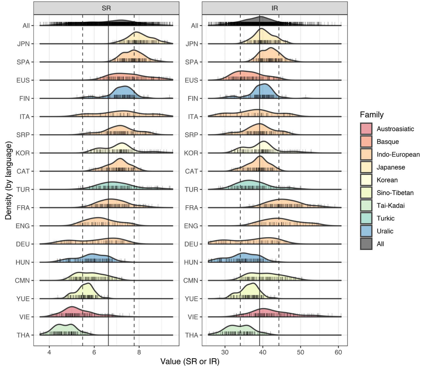
As it turns out, there’s less cross-linguistic variability in information rate than speech rate. This is depicted in the figure below. The panel on the left illustrates density plots (basically histograms) for the distribution over speech rates for each language. As you can see, there’s considerable variability: the modal speech rate for Japanese is about 1 standard deviation above the mean speech rate across languages, and pretty much the entire distribution of speech rates for Thai falls at least 1 standard deviation below the mean speech rate across languages.

The panel on the right illustrates the same thing, but for information rates. Even just visually, it’s clear that there’s less cross-linguistic variability. Most languages fall within 1 SD of the mean information rate (~39 bits/second). This inference is further backed up by several statistical comparisons of these measures.

Interpretation

The authors draw two important conclusions from these analyses.

First, they suggest that there’s a natural trade-off between speech rate and information density, as evidenced by the negative correlation between the two. The suggestion here is that speakers compensate–either automatically or strategically–for the information density of their language by either speaking faster (for information-sparse languages) or slower (for information-dense languages).

Second, they argue that this reflects some kind of universal biological constraint–i.e., that the human brain has some innate limitation on the amount of information it can process per second. Information-dense languages spoken too fast may exceed this “channel capacity”, while information-sparse languages spoken too slowly may incur a cost on working memory, and are generally less efficient. Thus, they argue that languages inhabit a stable, optimal region of information rates, constrained by this limitation.

Both conclusions are of great theoretical interest. They’re compatible with a perspective in which the evolution of languages is shaped by psychological and biological constraints of their speakers–and so while languages vary considerably along many dimensions, this variability will always be within some space defined by those constraints. Perhaps this high-level point seems obvious, but as always with these questions, the devil is in the details: what are those constraints, and which features are shaped by them? In this case, the authors argue for a constraint on “information-processing speed”, with information rate centered around 39 bits/second. This also opens the door to further work: what neural mechanisms underlie this constraint on information-processing, and what processes shape this compensatory trade-off between speech rate and information density?

Discussion: limitations and conclusions

What should we take away from this study? What limitations are there in the authors’ analysis and interpretation?

Limitation 1: is this about conditional entropy or just the number of possible syllables?

Recall that the authors’ measure of “information density” is the conditional entropy over syllables: given the syllable that came before, how much certainty do I have about the syllable the speaker is about to produce? As noted, this measure will depend on the number of possible syllables ⁶ in a language.

Thus, from the current analysis, it’s hard to know whether their finding is purely a function of the number of syllables in the language, or whether it’s really about syllable predictability specifically. The difference amounts to the difference between the two conclusions below:

Conclusion 1: Languages in which syllables are more predictable (lower conditional entropy) tend to be spoken faster than languages in which syllables are less predictable (higher conditional entropy).

Conclusion 2: Languages with less possible syllables tend to be spoken faster than languages with more possible syllables.

One way to adjudicate between these possibilities this would be to compare two languages with the same number of possible syllables (e.g., 50 syllables) but different conditional probability distributions over that space of syllables. If those languages don’t differ in their average speech rate, then we would know that the finding is consistent with conclusion 2. But if those languages do have different average speech rates–i.e., the high-entropy language is spoken slower than the low-entropy language–then the finding really does seem to be about syllable predictability per se.

Limitation 2: what is “information”?

Even if conclusion 1 above is true, there’s still a major limitation (in my view) regarding the inference that this is about information rate specifically.

In this post, I’ve tried to emphasize the difference between the technical meaning of “information”, as operationalized here, and the colloquial, everyday meaning. The notion of “information” in the paper amounts to the probability over signals in a communication system–i.e., how probable is one syllable vs. another, given the previous syllable? At least from my perspective, this is very different from my default interpretation of the word “information”, which is something like “information content”. I don’t think the uncertainty over signals is the same as the uncertainty over meanings.

Of course, meaning is hard to define. Pretty much any operationalization is unsatisfying in some way. That’s precisely why entropy is usually defined over signals, rather than meanings. I think this can be confusing, especially when results are translated to the public. Hopefully this post has highlighted some of that nuance–if only by showing that the meaning of “information” is more complicated than one might assume from a headline.

Limitation 3: what is “optimal”?

The last limitation I’ll discuss is higher-level, and concerns the authors’ conclusion that:

However, languages seem to stably inhabit an optimal range of IRs, away from the extremes that can still be available to individual speakers. Languages achieve this balance through a trade-off between ID and SR, resulting in a narrower distribution of IRs compared to SRs (pg. 5).

The cruciul finding in the paper is that variability in information rate is less than variability in speech rate. This may be evidence of a trade-off; but is it evidence of optimality?

First, how can one even define “optimality”? There’s a considerable amount of research in the field right now arguing that language is an optimal code for communication. Certainly, it’s clear that language evolution is shaped by the psychological, social, and biological pressures of the humans that learn, produce, and comprehend language. But does that really make it “optimal”, or just “good enough”? The process of natural selection in biological evolution doesn’t produce optimal organisms, but rather, organisms that are good enough to survive and reproduce in a particular ecosystem. To their credit, the authors acknowledge and even support this point:

We suggest that this valley in a fitness landscape illustrates the concept of “good-enough” control proposed as an alternative to optimal control for biological systems (34) and that its existence is due to functional and cognitive factors (pg. 5).

Where, then, does the notion of optimality enter? Judging from the analysis, it would seem that the optimal “attractor” for information rate is 39 bits/second–i.e., the mean information rate across languages. But this raises a second point: languages may vary less in information rate than speech rate, but there’s still considerable variability around the mean. Some languages (like Thai) still have a modal information rate about 1 SD below the mean. I don’t think the authors would argue that Thai is somehow less optimal than English or Japanese. But that raises the question: what factors contribute to a language’s position in this “fitness landscape”?

Takeaway

Hopefully the discussion of limitations above does not detract from the strengths of the paper. It’s quite interesting that languages in which syllables are more predictable are spoken faster than languages in which syllables are less predictable. It’s also very exciting that the authors found a feature that demonstrates less variability than most other linguistic features. As noted in the introduction, finding features of language that appear to be invariant across languages gives us insight into the origins of language and into the biological constraints shaping language evolution. This finding also establishes a promising research program investigating the mechanisms underlying these possible trade-offs.

My focus on the limitations is driven primarily by a desire to clarify some of the terminology–in particular, the meaning of “information”. Words mean different things in different contexts, and it’s important to remember that a scientific use of a term isn’t always the same as our intuitive understanding of that word ⁷.

Footnotes

References

Coupé, C., Oh, Y. M., Dediu, D., & Pellegrino, F. (2019). Different languages, similar encoding efficiency: Comparable information rates across the human communicative niche. Science Advances, 5(9), eaaw2594.

Cohen Priva, U. (2017). Informativity and the actuation of lenition. Language, 93(3), 569-597.

Piantadosi, S. T., Tily, H., & Gibson, E. (2012). The communicative function of ambiguity in language. Cognition, 122(3), 280-291.

Shannon, C. E. (1948). A mathematical theory of communication. Bell system technical journal, 27(3), 379-423.