
P-hacking in R [stats]
Introduction
The goal of most scientific research is knowledge construction. This typically involves investigating potential relationships between variables of interest (does A relate to B?), especially causal relationships (does A cause B?).
One way to investigate a relationship between two or more variables is through experimentation. In the classical model of research, a scientist formulates a hypothesis (A/~A causes some change in B), designs an experiment to test that hypothesis (usually by parametrically maniuplating A), collects data, and analyzes that data using some kind of statistical test.
All stages of this standard pipeline are subject to critical errors of reasoning. In this post, I’ll focus on challenges that arise during analysis, but many of the insights actually apply to other stages as well. Specifically, this post will demonstrate the problem of researcher degrees of freedom.
Researcher degrees of freedom
Researchers generally have considerable flexibility in the design and analysis of their experiments. Importantly, these “degrees of freedom” often go unreported, and also aren’t incorporated into a researcher’s interpretation of their results.
To understand exactly why this is problematic, it’s necessary to briefly explain the logic of null hypothesis significance testing (NHST).
What is NHST?
Many scientists analyze their data using a null hypothesis significance test. Philosophically, this involves comparing an alternative hypothesis (A relates to B) to the null hypothesis: the hypothesis of “no effect or no relationship based on a given observation” (Pernet, 2015).
This usually involves computing some measure of the difference in a dependent variable (B) across conditions (A/~A), then calculating a p-value: the probability of observing a result this extreme under the null hypothesis (James et al, 2013). As Pernet (2015) notes, a p-value is explicitly not an indication of the magnitude of an effect, nor does it explicitly favor a given hypothesis or allow a researcher to calculate the probability of replicating an effect. It is simply the probability––usually conditioned on some assumption of normality––of observing a result this extreme, if the null hypothesis (e.g., no difference across conditions) were true.
There are many issues that arise when scientists focus primarily on p-values. As McShane et al (2019) point out, scientists often treat p-values as categorical thresholds—p < .05 is “significant”, p > .05 is “not significant”—even though the underlying value, of course, is continuous. There are also considerable debates around the appropriate thresholds (fuzzy or otherwise) with which to evaluate these metrics (Benjamin et al, 2018).
Here, I’ll focus on an issue that arises when scientists ignore a core assumption of p-values, and NHST more generally. A fundamental assumption of NHST is that scientists develop a hypothesis before collecting and analyzing their data. Unfortunately, this assumption is often violated in practice, as in the case of p-hacking.
P-hacking
The more statistical analyses a researcher runs—the more hypotheses they “test”—the more likely that at least one of these analyses will produce a result that appears to be “significant”, simply by chance. Lots of things in the world are spuriously correlated. If you compare 1000 variables at random, there’s a pretty high probability that at least 1-2 of these variables will be related.
In principle, there’s nothing wrong with exploratory data analysis. It probably shouldn’t be totally random, but in the age of “Big Data”, more and more scientific research involves using machine learning to mine potentially significant results from high-dimensional datasets. Couched appropriately (e.g., as a method to generate potential hypotheses for further experimentation) this is actually a critical part of the scientific process.
The problem is that researchers don’t always interpret these results with appropriate caution. They present the results of exploratory research as if they were confirmatory—reporting only the results that turned out significant, and acting as if those specific hypotheses were developed from the beginning.
P-hacking is a huge problem for science because it makes it difficult to trust a researcher’s results. How many tests did a researcher need to run before they “discovered” this particular finding? How many times did they split their data (e.g., “Does A affect B in men between the ages of 30-35? What about between 35-40?”)?
A simulation-based demonstration of p-hacking
Maybe the claim that simply running more statistical tests will yield an apparently significant finding seems suspicious to you.
Fortunately, it’s pretty simple to demonstrate this empirically. We can simulate two random distributions (X and Y), which we have no a priori reason to believe are related. By shuffling X a number of times, we can simulate the process of exploring other random variables that may or may not be related to Y. On each shuffle, we compare our new X to our dependent variable Y using a statistical test (e.g., linear regression). Finally, we look at our distribution of coefficients and p-values, and ask whether any of these “findings” fall below the standard significance threshold.
Simulating our data
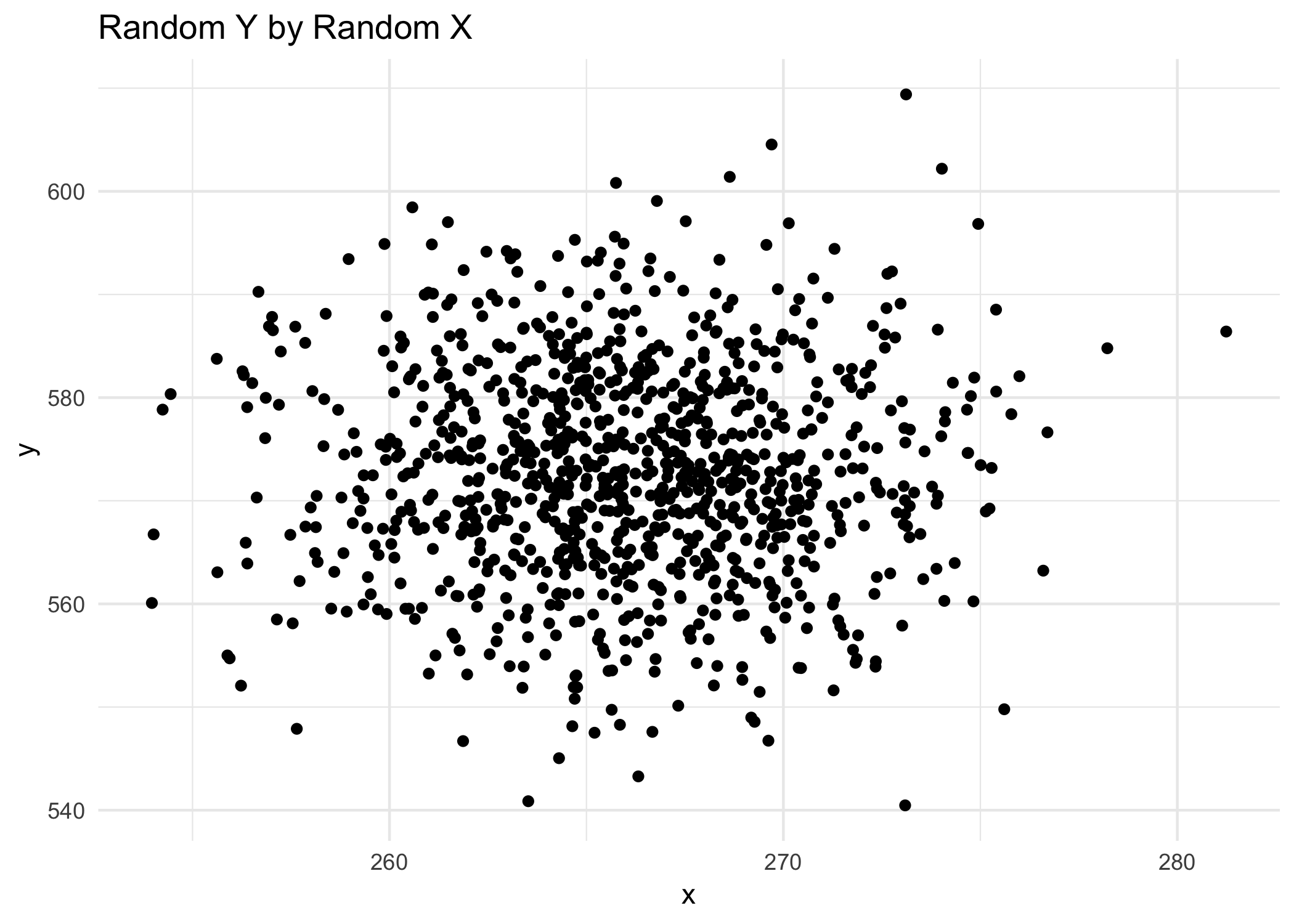
First, we set up our two random datasets. Here, X and Y are constructed as normal distributions centered around some means (X_MEAN, Y_MEAN), each with standard deviations falling between [1, 10].
set.seed(1)

X_MEAN = sample(1:1000, 1)
X_SD = sample(1:10, 1)
Y_MEAN = sample(1:1000, 1)
Y_SD = sample(1:10, 1)

x = rnorm(1000, mean=X_MEAN, sd=X_SD)
y = rnorm(1000, mean=Y_MEAN, sd=Y_SD)

og_data = data.frame(x=x, y=y)
We can then plot this data. It’s pretty clear that there’s no relationship between X and Y.
og_data %>%
  ggplot(aes(x = x,
             y = y)) +
  geom_point() +
  theme_minimal() +
  labs(title = "Random Y by Random X")
Hacking the data
Now we can simulate p-hacking by shuffling our X a number of times (here, NUM_HACKS=1000). On each shuffle, we regress Y ~ X'.
NUM_HACKS = 1000

test_coef = c()
test_p = c()
size_v = c()
for (i in c(1:NUM_HACKS)) {
  new_x = sample(x)
  # new_x = rnorm(1000, mean=X_MEAN, sd=X_SD)
  new_test = summary(lm(y ~ new_x))
  test_coef[i] = new_test$coefficients[2]
  test_p[i] = new_test$coefficients[8]
}

d = data.frame(coef = test_coef,
               p = test_p)
Finally, we can plot the distribution of coefficients (e.g., the slope of the best-fitting line between a given X' and Y) and their corresponding p-values.
d %>%
  ggplot(aes(x = test_coef,
             y = test_p)) +
  geom_point() +
  geom_hline(yintercept = .05, linetype = "dotted") +
  labs(x = "Coefficient",
       y = "P-value",
       title = "Statistics for randomly shuffled splits") +
  theme_minimal()
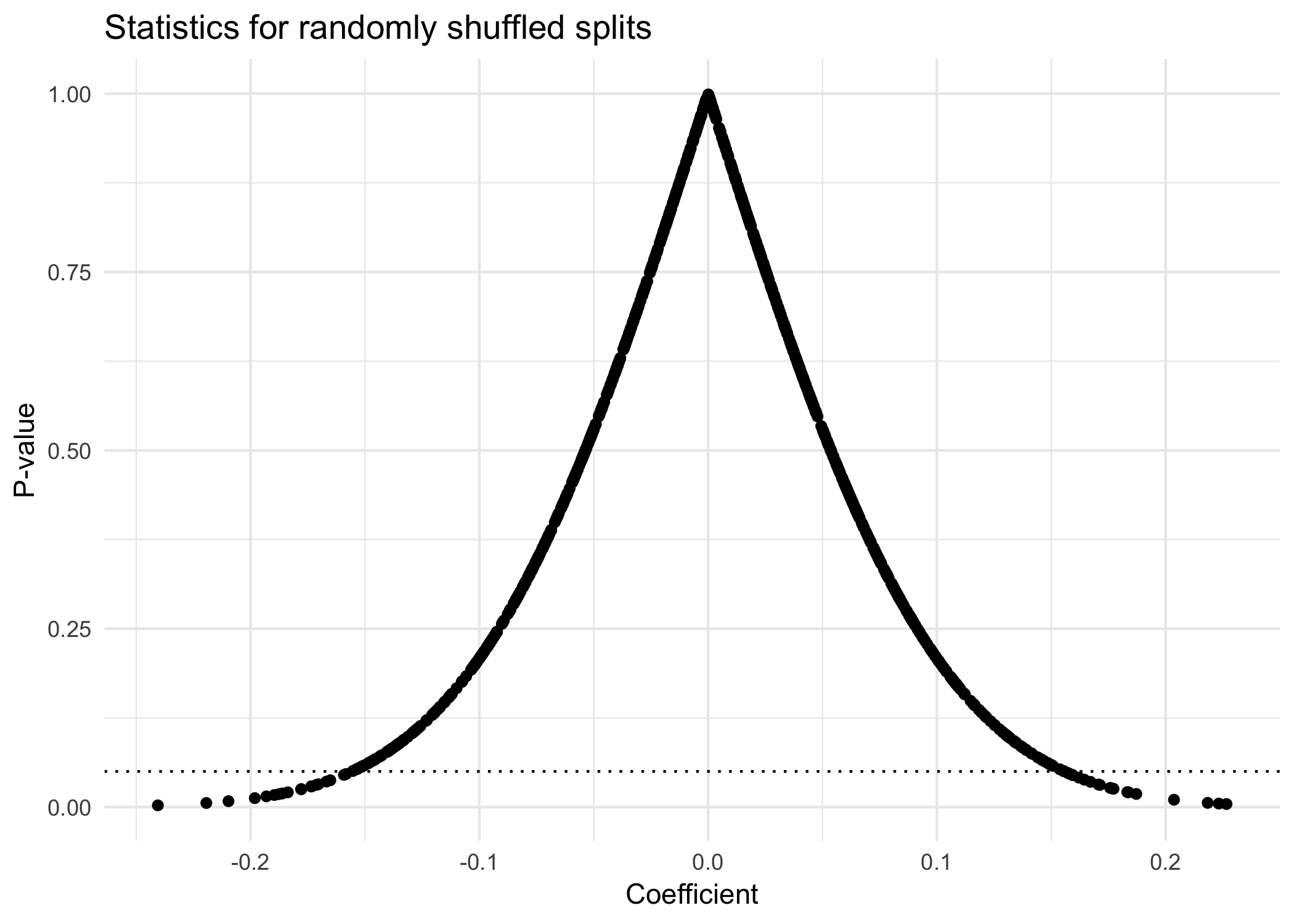
nrow(filter(d, test_p < .05))/nrow(d)
## [1] 0.039
Looking at the plot above, we see that while most of our p-values fall above the dotted line (p=.05), some do not. Specifically, almost 4% have a p-value below .05. According to the standard significance threshold, these values are “significant”.
Of course, we know—having simulated the data—that these results are simply the result of random shuffling. The vast majority of these 1000 random shuffles produced uncorrelated data. If we reported all of these tests, there wouldn’t be a problem; it’d be clear that the few “significant” findings were due to random chance. But if we reported only the 4% with p<.05, it would appear to readers that these were the only tests we ran, and thus that these findings really were meaningful.
Code availability
The code above is a simulation-based demonstration that the more randomly-generated datasets you compare, the more likely you are to find something that’s correlated.
Of course, there are a number of parameters that can be adjusted in the code above, including:
- The random seed (currently set to 1)
- Both
X_MEANandY_MEAN - Both
X_SDandY_SD - The number of comparisons (
NUM_HACKS=1000) - The kind of distribution you’re sampling from for both
XandY(currently a normal distribution) - The decision to either shuffle the original
Xor generate a newXeach time
I encourage you to try varying any and all of them. You can find the full code sample here, which you can run in R. Note that this code also includes a parameter called SUBGROUP_SIZE; in addition to running NUM_HACKS comparisons, this code sub-samples from X and Y for each comparison, which is meant to be analogous to splitting one’s data.
Also, if you have R Studio with shiny equipped, you can also download a shiny script here, which you can run interactively in your browser to dynamically change the parameters above.
Potential solutions
Researcher degrees of freedom pose a serious problem for ethical, trustworthy science. Many researchers can even fool themselves into thinking a post-hoc analysis was planned all along, simply because the motive is so strong—after all, a significant result is more likely to be published, and publications are critical for career development in academia.
Fortunately, there’s a large (and growing) community of scientists, journalists, and others who are invested in solving this problem. There’s the Center for Open Science, the Society for the Improvement of Psychological Science, the Open Science Framework, or OSF, and more. P-hacking is far from the only issue of concern in this community, but it is one that people have thought seriously about.
Two of the solutions that most appeal to me are:
- Pre-registration: basically, a researcher can “pre-register” all the relevant details of their intended analysis, even including the script they plan to use to analyze the data, using a site like OSF. This doesn’t preclude the researcher from conducting later exploratory analyses, but it’s clear to both the researcher and possible reviewers which analyses were planned, and which were conducted during post-hoc exploration of the data.
- Multiverse analysis: as Steegen et al (2019) describe, each step of the analysis pipeline involves a series of (sometimes arbitrary) decisions made by the researchers. This effectively creates a “multiverse” of possible analyses. The authors suggest committing to this multiversality; instead of only testing one operationalization, one analysis, researchers can test many, and ask about how robust a given result is across all of these analyses. This approach can reveal that particular results are very fragile, e.g., very dependent on a particular choice of statistical model or subset of the data.
In my view, these solutions are mutually compatible. Pre-registration is a concrete mechanism to hold researchers accountable, both to the community and to themselves. And a multiverse analysis acknowledges the probabilistic and contingent nature of scientific truth. Ultimately, our goal is to construct useful models that explain the world around us, and it’s important that we do so honestly and transparently.
Contact
Of course, if you have questions, comments, or criticisms about this post, you can contact me at sttrott at ucsd dot edu.
References
Benjamin, D. J., Berger, J. O., Johannesson, M., Nosek, B. A., Wagenmakers, E. J., Berk, R., … & Cesarini, D. (2018). Redefine statistical significance. Nature Human Behaviour, 2(1), 6.
Pernet, C. (2015). Null hypothesis significance testing: a short tutorial. F1000Research, 4.
McShane, B. B., Gal, D., Gelman, A., Robert, C., & Tackett, J. L. (2019). Abandon statistical significance. The American Statistician, 73(sup1), 235-245.
Steegen, S., Tuerlinckx, F., Gelman, A., & Vanpaemel, W. (2016). Increasing transparency through a multiverse analysis. Perspectives on Psychological Science, 11(5), 702-712.