Note: This post attempts to summarize part of Chapter 6 from “Introduction to Statistical Learning” (James et al, 2013); the full textbook can be found here in PDF form, which contains a number of examples and walks through the equations in more detail.

Introduction

In science, we try to explain the world in terms of relationships between different theoretical constructs. These explanations are often grounded in the language of statistical models, e.g.: “Variable X1 relates to changes in Y in the following way, while X2 relates to changes in Y in a different way.” Sometimes we intend these explanations to be causal, though the step to causal inference can be theoretically fraught. Most broadly, the role of these statistical models is to provide some kind of quantitative description of the relationship between our variables of interest (whether causal or otherwise).

This often amounts to a regression problem: we want to estimate the coefficients on a set of variables that relate to linear (or in some cases, nonlinear) changes in Y. A common form of linear regression is ordinary least squares (OLS): given a matrix of predictors X, we estimate coefficients (or “weights”) for each variable {X1, ..., Xp} (where p=number of predictors), such that we minimize the error between our predicted values and the observed values of Y. Put simply, we draw a line that best fits our data.

This approach is intuitive, but it does carry with it a set of problems. In particular, as the number of potential predictors increases, models become both less interpretable and more prone to overfitting––that is, our model achieves a better fit to the data, but will likely suffer from a lack of generalizability. This becomes especially problematic as the number of predictors approaches the number of observations in our dataset. As James et al (2013) suggest, one solution to overfitting is subset selection: identify the subset of predictors that have “significant” relationships to your outcome variable. This can be done using either metrics of model fit (AIC, BIC, adjusted R2, etc.), and/or by asking about how well the model generalizes to a test set.

Another approach, which I’ll focus on here, is regularization: instead of fitting subsets of our predictors, we can fit all of them, but impose something called a shrinkage penalty––basically, we “shrink” the coefficient values for our predictors, which ultimately reduces their variance. In the case of Lasso regression, this can be used to force most of the coefficients to 0 (effectively rendering them irrelevant); thus, the relevant predictors are those which have non-zero coefficients.

An intuitive explanation of Lasso regression: Regularization as “budgeting”

The way I understand Lasso regression (and other regularization approaches like ridge or elastic net) is that they’re just extensions of the OLS formula:

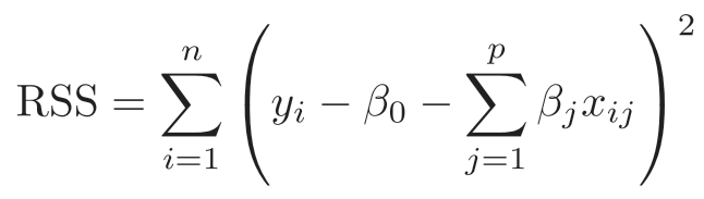
In OLS regression, we try to minimize the residual sum of squares (RSS), e.g. the error between our predicted values and our actual values. The formula for deriving the RSS is given below. In plain English, this translates to: for each data point, subtract from the actual value (y-real) the intercept (b0, e.g. the prediction when all predictors=0), as well as the predicted value y-pred (obtained by summing the product of our x by the coefficient for each predictor). Critically, we want to minimize this value. This is intuitive when you consider it from the perspective of identifying the best explanation for your data––you want to estimate the relationships between X and Y that, when applied to X, best predict Y.

Lasso regression uses OLS regression as its starting point (see the left-side of the equation below), but adds a shrinkage penalty term.

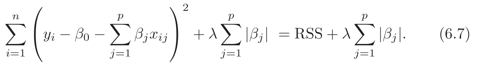
Specifically, in addition to minimizing the RSS, we want to minimize the sum of the absolute values of our coefficients.

Note the curious l in our shrinkage penalty term. This is called a tuning parameter (“lambda”), and its value essentially determines the extent to which we impose this penalty. If l=0, the equation reduces to standard OLS regression. But as l increases, we impose a stricter and stricter penalty––we force more and more of our coefficients to be smaller, creating a sparse vector of non-zero coefficients.

What’s the intuition behind this approach? James et al (2013) describe regularization as a kind of budget. Like with standard OLS regression, we’re still trying to find the model that best fits our data, but we’re working under an additional budgetary constraint: we can’t assign too much “credit” to our variables. And the larger our l term, the stricter our budget. This has the beneficial effect of shrinking our coefficient estimates towards 0, allowing us to identify the most relevant (e.g. non-zero) set of predictors that remain (according to the model).

Why use regularization?

As described above, Lasso regularization is particularly useful for feature selection: you have a large set of predictors, and you want to isolate the predictors that are truly related to your Y.

This kind of approach is becoming increasingly relevant, as the size of our datasets increases. This approach is useful in fields such as Genetics, Economics, and Epidemiology, all of which involve building large, multivariate models. Regularization is also useful in machine learning, and is often used in conjunction with techniques such as cross-validation, in order to build models that incorporate many potential predictors but weight only a subset of these predictors, in order to generalize across limited training sets.

James et al (2013) also describe a number of other regularization approaches, including ridge regression. Ridge is similar to Lasso, but rather than minimizing the sum of your coefficient values, you minimize the sum of the squared coefficient values. This seemingly small difference actually results in some profound differences in how the models work––ridge regression never shrinks any coefficients entirely to 0. As James et al (2013) note, ridge regression is thus equivalent to assuming that your coefficients are randomly distributed around 0, whereas Lasso regression is equivalent to assuming that many of your coefficients equal 0.

References

James, G., Witten, D., Hastie, T., & Tibshirani, R. (2013). An introduction to statistical learning (Vol. 112, p. 18). New York: springer.