The \(R^2\), or coefficient of determination, measures the proportion of variance in \(Y\) explained by the model.
\(R^2 = 1 - \frac{RSS}{SS_Y}\)
Where \(SS_Y\) is the sum of squared error in \(Y\).
💭 Check-in
What does this formula mean and why does it measure the proportion of variance in \(Y\) explained by the model?
Decomposing \(R^2\)
\(R^2 = 1 - \frac{RSS}{SS_Y}\)
\(RSS\) refers to the unexplained (residual) variance in \(Y\) from the model.
\(SS_Y\) is the total variance in \(Y\) (i.e., before even fitting the model).
Thus, \(\frac{RSS}{SS_Y}\) captures the proportion of unexplained variance by the model.
If \(\frac{RSS}{SS_Y} = 1\), the model has explained no variance.
If \(\frac{RSS}{SS_Y} = 0\), the model has explained all variance.
And \(1 - \frac{RSS}{SS_Y}\) captures the proportion of explained variance.
Key assumptions of linear regression
Ordinary least squares (OLS) regression has a few key assumptions.
Assumption
What it means
Why it matters
Linearity
The relationship between \(X\) and \(Y\) is linear
OLS fits a straight line, so if the true relationship is curved, predictions will be systematically biased
Independence
The observations are independent of each other
Dependent observations (e.g., repeated measures, time series) violate the assumption that errors are uncorrelated, leading to underestimated standard errors and invalid p-values
Homoscedasticity
The variance of residuals is constant across all levels of \(X\) (equal spread)
If variance changes with \(X\) (heteroscedasticity), standard errors will be incorrect: some coefficients appear more/less significant than they truly are
Normality of residuals
The errors are approximately normally distributed
Needed for valid confidence intervals and hypothesis tests (p-values). Less critical with large samples due to the Central Limit Theorem.
Interim summary
In statistical modeling, we aim to construct models of our data.
Linear regression is a specific (high-bias) model.
The goal of linear regression is to identify the best-fitting line for our data, i.e., to reduce the residual sum of squares (RSS).
Linear regression rests on a few assumptions about the data (more on this in an upcoming lecture).
Part 3: Linear regression in R
Using and interpreting fit lm models, using broom.
The lm function
A linear model can be fit using the lm function.
Supply a formula (i.e., y ~ x).
Supply the data (i.e., a dataframe).
Usage: lm(data = df_name, y ~ x).
Where y and x are columns in df_name.
Loading a dataset
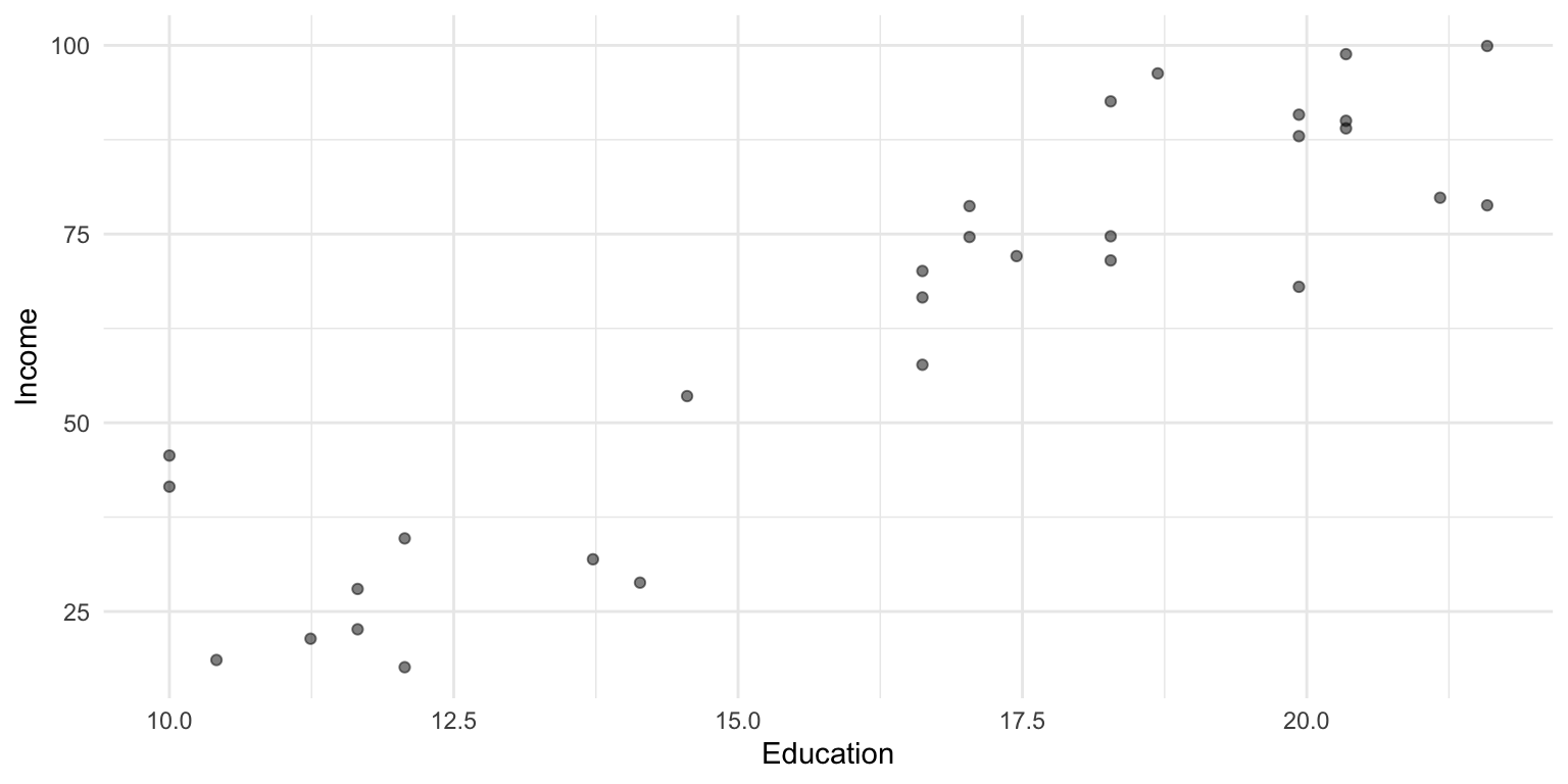
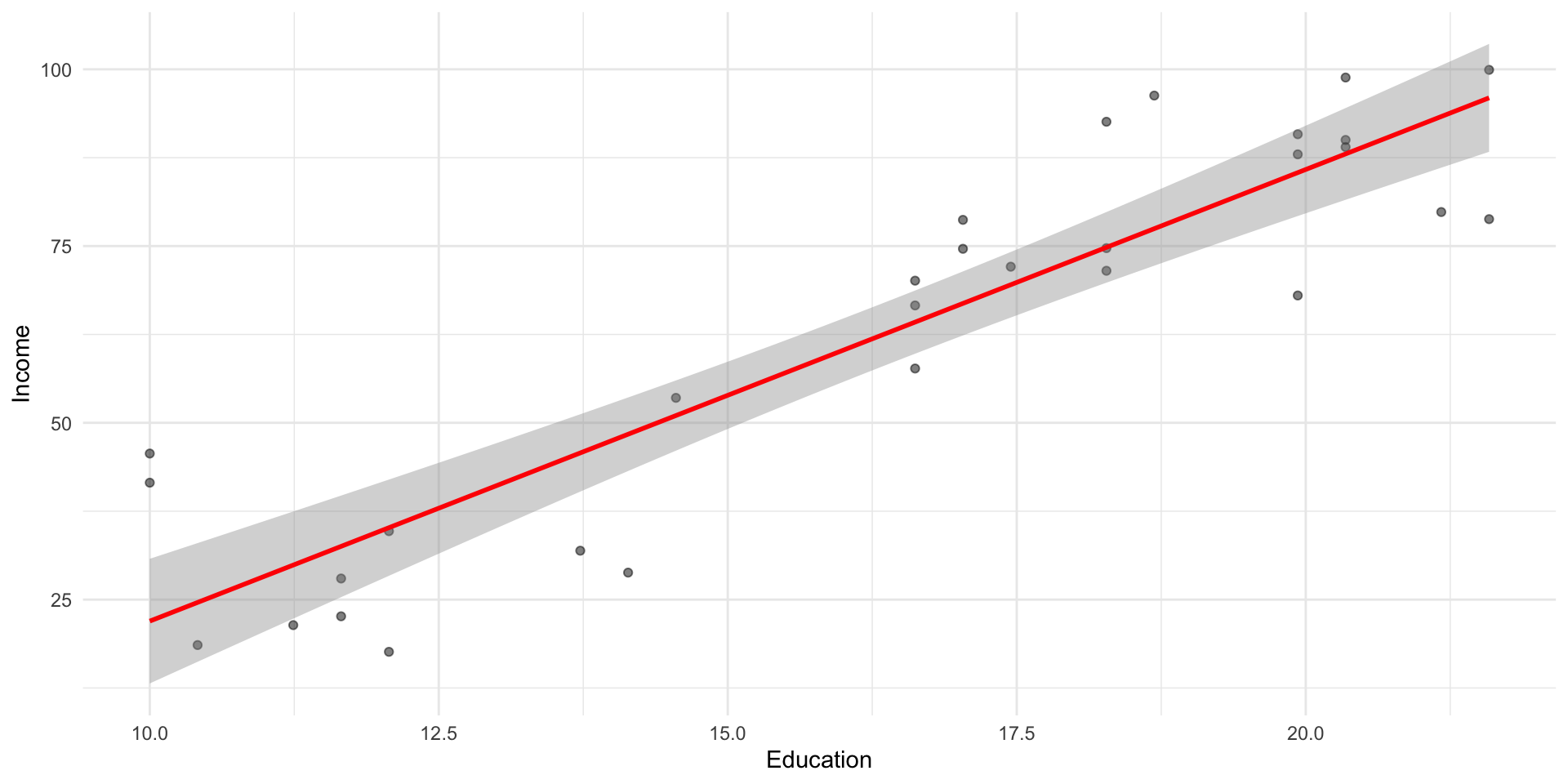
To illustrate linear regression in R, we’ll work with a sample dataset.
As we discussed before, geom_smooth(method = "lm") can be used to plot a regression line over your data.
df_income %>%ggplot(aes(x = Education, y = Income)) +geom_point(alpha = .5) +geom_smooth(method ="lm", se =TRUE, color ="red") +theme_minimal()
Tip
But to actually fit a model, we need to use lm.
Fitting an lm model
Calling summary on a fit lm model object returns information about the coefficients and the overall model fit.
mod =lm(data = df_income, Income ~ Education)summary(mod)
Call:
lm(formula = Income ~ Education, data = df_income)

Residuals:
    Min      1Q  Median      3Q     Max
-19.568  -8.012   1.474   5.754  23.701

Coefficients:
            Estimate Std. Error t value Pr(>|t|)
(Intercept) -41.9166     9.7689  -4.291 0.000192 ***
Education     6.3872     0.5812  10.990 1.15e-11 ***
---
Signif. codes:  0 '***' 0.001 '**' 0.01 '*' 0.05 '.' 0.1 ' ' 1

Residual standard error: 11.93 on 28 degrees of freedom
Multiple R-squared:  0.8118,    Adjusted R-squared:  0.8051
F-statistic: 120.8 on 1 and 28 DF,  p-value: 1.151e-11
Understanding summary output
Calling summary returns information about the coefficients of our model, as well as indicators of model fit.
summ =summary(mod) summ$coefficients
              Estimate Std. Error   t value     Pr(>|t|)
(Intercept) -41.916612  9.7689490 -4.290801 1.918257e-04
Education     6.387161  0.5811716 10.990148 1.150567e-11
summ$r.squared
[1] 0.8118069
Estimate: fit intercept and slope coefficients.
Std. Error: estimated standard error for those coefficients.
t value: the t-statistic for those coefficients (slope / SE).
p-value: the probability of obtaining a t-statistic that large assuming the null hypothesis.
Multiple R-squared: proportion of variance in y explained by x.
Residual standard error: The standard error of the estimate.
Interpreting coefficients
There are a few relevant things to note about coefficients:
The estimate tells you the direction (sign) and degree (magnitude) of the relationship.
The p-value tells you whether a relationship of this size would be expected assuming there was no effect (i.e., the null hypothesis).
More on this in an upcoming lecture!
💭 Check-in
How would you report and interpret the intercept and slope we obtained for Income ~ Education? (As a reminder, \(\beta_0 = -41.9\) and \(\beta_1 = 6.4\).)
The broom package
The broom package is also an easy way to quickly (and tidily) extract coefficient estimates.
How might you model and interpret the effect of a categorical variable?
Contrast coding
A common approach is to use the mean of one level (e.g., Congruent) as the intercept; the slope then represents the difference in means across those levels.
### Actual meansdf_stroop %>%group_by(Condition) %>%summarise(mean_RT =mean(RT))