Regression: Advanced Issues
Goals of the lecture
- Multiple regression: beyond single predictors.
- Modeling interaction effects.
- Advanced topics in regression:
- Understanding standard errors and coefficient sampling distributions.
- Heteroscedasticity.
- Multicollinearity.
Part 1: Multiple regression
Multiple predictors, interpreting coefficients, and interaction effects.
What is multiple regression
Multiple regression means building a regression model (e.g., linear regression) with more than one predictor.
There are a few reasons to do this:
- Multiple predictors helps “adjust for” multiple correlated effects, i.e., \(X_1\) and \(X_2\).
- Tells us the effect of \(X_1\) on \(Y\), holding constant the effect of \(X_2\) on \(Y\).
- Important for addressing confounding variables.
- In general, adding more predictors often results in more powerful models.
- Better for predicting things in the real world!
Loading a dataset
Fortunately, we can still use lm to build multiple regression models in R. To get started, let’s load the income dataset we used in previous lecutres.
[1] 30Building a multiple regression model
To add multiple predictors to our formula, simply use the + syntax.
Call:
lm(formula = Income ~ Seniority + Education, data = df_income)

Residuals:
   Min     1Q Median     3Q    Max
-9.113 -5.718 -1.095  3.134 17.235

Coefficients:
             Estimate Std. Error t value Pr(>|t|)
(Intercept) -50.08564    5.99878  -8.349 5.85e-09 ***
Seniority     0.17286    0.02442   7.079 1.30e-07 ***
Education     5.89556    0.35703  16.513 1.23e-15 ***
---
Signif. codes:  0 '***' 0.001 '**' 0.01 '*' 0.05 '.' 0.1 ' ' 1

Residual standard error: 7.187 on 27 degrees of freedom
Multiple R-squared:  0.9341,    Adjusted R-squared:  0.9292
F-statistic: 191.4 on 2 and 27 DF,  p-value: < 2.2e-16
💭 Check-in
Try building two models with each of those predictors on their own. Compare the coefficient values and \(R^2\). Any differences?
Comparing coefficients to single predictors
In general, we see that the coefficients are pretty similar from the single-variable models and the multiple-variable models, though generally reduced in the multiple-variable model.
# Model 1: Single predictor - Seniority only
mod_seniority <- lm(Income ~ Seniority, data = df_income)
# Model 2: Single predictor - Education only
mod_education <- lm(Income ~ Education, data = df_income)
# Model 3: Multiple regression - Both predictors
mod_multiple <- lm(Income ~ Seniority + Education, data = df_income)

mod_seniority$coefficientsComparing fit to single predictors
We also see that the model with multiple predictors achieves a better \(R^2\).
[1] 0.2686226[1] 0.8118069[1] 0.9341035💭 Check-in
Are there any potential concerns with using standard \(R^2\) here?
Using adjusted R-squared
Adjusted \(R^2\) is a modified version of \(R^2\) that accounts for the fact that adding more variables will always slightly improve model fit.
\(R^2_{adj} = 1 - \frac{RSS/(n - p - 1)}{SS_Y/(n - 1)}\)
Where:
- \(n\): number of observations.
- \(p\): number of parameters in model.
[1] 0.242502[1] 0.8050857[1] 0.9292223Note
As \(p\) increases, the numerator decreases, i.e., it’s a penalty for adding more predictors.
AIC: Another metric of fit
Akaike Information Criterion (or AIC) is another commonly used metric of model fit.
\(AIC = 2k - 2\ln(L)\)
Where:
- \(k\) is the number of parameters.
- \(L\) is the likelihood of the data under the model (we’ll discuss this soon!).
Note
Unlike \(R^2\), a lower AIC is better. We’ll talk more about model likelihood later in the course!
Your turn: using mtcars
Now, let’s apply this using the mtcars dataset:
- Try to predict
mpgfromwt. Interpret the coefficients and model fit. - Then try to predict
mpgfromam. Interpret the coefficients and model fit. Note that you might need to convertaminto a factor first. - Finally, predict
mpgfrom both variables. Interpret the coefficients and model fit.
Writing out the linear equation
It’s often helpful to practice writing out the linear equations for a fit lm. Let’s write out the equations for the multiple variable model above.
\(Y_{mpg} = 37.32 - 5.35X_{wt} - 0.02X_{am}\)
💭 Check-in
What about interactions between our terms?
Interaction effects
An interaction effect occurs when the effect of one variable (\(X_1\)) depends on the value of another variable (\(X_2\)).
- So far, we’ve assumed variables have roughly additive effects.
- An interaction removes that assumption.
- In model, allows for \(X_1 * X_2\), i.e., a multiplicative effect.
Examples of interaction effects
Any set of variables could interact (including more than two!), but it’s often easiest to interpret interactions with categorical variables.
Food x Condiment: The enjoyment of aFood(ice cream vs. hot dog) depends on theCondiment(Chocolate vs. Ketchup).Treatment x Gender: The effect of some treatment depends on theGenderof the recipient.Brain Region x Task: The activation in differentBrain Regionsdepends on theTask(e.g., motor vs. visual).
Building an interaction effect
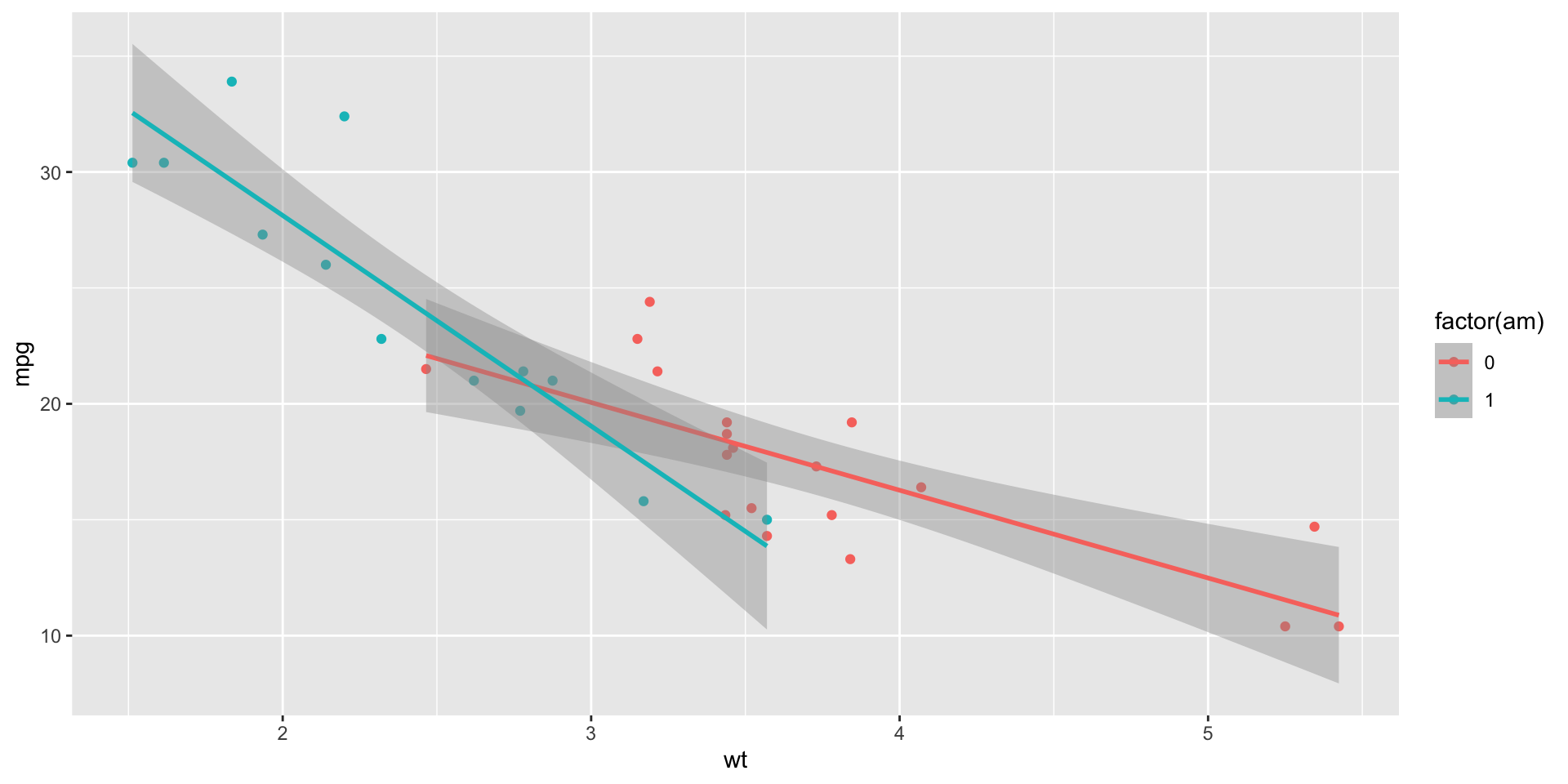
We can interpret the coefficients as follows:
- Intercept: Automatic cars (
am = 0) withwt = 0have expectedmpgof 31. wt: Aswtincreases, we expect automatic cars to decreasempgby about 3.7.factor(am): Holdingwtconstant, manual cars have an expectedmpgof about 14 more than automatic cars.- Interaction: Among manual cars, increases in
wtcorrespond to even sharper declines in expectedmpg.
Call:
lm(formula = mpg ~ am * wt, data = mtcars)

Residuals:
    Min      1Q  Median      3Q     Max
-3.6004 -1.5446 -0.5325  0.9012  6.0909

Coefficients:
            Estimate Std. Error t value Pr(>|t|)
(Intercept)  31.4161     3.0201  10.402 4.00e-11 ***
am           14.8784     4.2640   3.489  0.00162 **
wt           -3.7859     0.7856  -4.819 4.55e-05 ***
am:wt        -5.2984     1.4447  -3.667  0.00102 **
---
Signif. codes:  0 '***' 0.001 '**' 0.01 '*' 0.05 '.' 0.1 ' ' 1

Residual standard error: 2.591 on 28 degrees of freedom
Multiple R-squared:  0.833, Adjusted R-squared:  0.8151
F-statistic: 46.57 on 3 and 28 DF,  p-value: 5.209e-11
Visualizing an interaction
By default, R will draw different regression lines for each level of a categorical factor we’ve added an aes for.
Interim summary
- Multiple regression models are often more powerful than single-variable models.
- In some cases, adding an interaction helps account for relationships that depend on another variable.
- But adding multiple variables does make interpretation slightly more challenging.
Part 2: Advanced topics
Standard errors, heteroscedasticity, and multicollinearity.
Coefficient standard errors (SEs)
The standard error of a coefficient measures the uncertainty in the estimated coefficient value.
When we inspect the output of a fit lm model, we can see not only the coefficients but the standard errors (Std. Error):
Call:
lm(formula = Income ~ Education, data = df_income)

Residuals:
    Min      1Q  Median      3Q     Max
-19.568  -8.012   1.474   5.754  23.701

Coefficients:
            Estimate Std. Error t value Pr(>|t|)
(Intercept) -41.9166     9.7689  -4.291 0.000192 ***
Education     6.3872     0.5812  10.990 1.15e-11 ***
---
Signif. codes:  0 '***' 0.001 '**' 0.01 '*' 0.05 '.' 0.1 ' ' 1

Residual standard error: 11.93 on 28 degrees of freedom
Multiple R-squared:  0.8118,    Adjusted R-squared:  0.8051
F-statistic: 120.8 on 1 and 28 DF,  p-value: 1.151e-11
💭 Check-in
Does a larger SE correspond to more or less uncertainty about our estimate?
The sampling distribution of coefficients
- If we could repeatedly sample from our population and fit our model each time, we’d get a distribution of coefficient estimates.
- This is called the sampling distribution of the coefficient.
- The standard error is the standard deviation of this sampling distribution.
- It tells us: “If we repeated this study many times, how much would our coefficient estimate vary?”
💭 Check-in
Which properties affect the standard deviation of that sampling distribution?
Calculating the SE
For a simple linear regression, the SE of the slope coefficient is:
\(SE(\beta_1) = \sqrt{\frac{\sum(y_i - \hat{y}_i)^2}{(n-2)\sum(x_i - \bar{x})^2}}\)
- Numerator: Larger residuals → more uncertainty → larger SE
- Denominator: More data points and more spread in \(X\) → less uncertainty → smaller SE
- For multiple regression, the calculation is more complex (involves matrix algebra)
- Fortunately, R calculates this for us!
Note
You will not be expected to calculate this from scratch!
The t-statistic
The t-statistic measures how many standard errors a coefficient is away from zero.
\(t = \frac{\hat{\beta} - 0}{SE(\hat{\beta})}\)
[1] 10.99015This matches the t value column in our summary output!
Interpreting the t-statistic
- The t-statistic follows a t-distribution under the null hypothesis that \(\beta = 0\).
- Rule of thumb: \(|t| \geq 2\) typically indicates statistical significance (p < 0.05).
- More precisely: We calculate the probability of observing a \(|t|\) this large (or larger) if the true coefficient were zero.
- This probability is the p-value.
💭 Check-in
Looking at our mod_education output, is the Education coefficient significantly different from zero?
Confidence intervals
We can use the SE to construct confidence intervals around our coefficient estimates:
\(\hat{\beta} \pm t_{critical} \times SE(\hat{\beta})\)
                 2.5 %     97.5 %
(Intercept) -61.927397 -21.905827
Education     5.196685   7.577637
Your turn: SEs and t-statistics
Using your mtcars model from earlier predicting mpg from wt and am:
- Which coefficient has the largest standard error?
- Which coefficient has the smallest p-value (most significant)?
- Calculate 99% confidence intervals using
confint(model, level = 0.99).
Heteroscedasticity
Heteroscedasticity occurs when the variance of residuals is not constant across all levels of the predictors.
- Homoscedasticity (the ideal): Residuals have constant variance.
- Heteroscedasticity (a problem): Residual variance changes with predictor values.
- This violates one of the key assumptions of linear regression!
- Consequences: Standard errors become unreliable, affecting our hypothesis tests.
💭 Check-in
Why would heteroscecasticity affect our interpretation of standard errors?
Heteroscedasticity and prediction error
The standard error of the estimate gives us an estimate of how much prediction error to expect.
- With homoscedasticity, our expected error shouldn’t really depend on \(X\).
- But with heteroscedasticity, our margin of error might actually vary as a function of \(X\).
- Yet we only have a single estimate of our prediction error, which might overestimate or underestimate error for a given \(X\) value.
Why heteroscedasticity biases SEs
The key insight:
- OLS gives equal weight to all observations when estimating SEs.
- But with heteroscedasticity, some observations have more noise than others.
- High-variance observations should be trusted less, but OLS doesn’t know this.
- Result: SEs don’t accurately reflect true uncertainty.
Detecting heteroscedasticity
We can diagnose heteroscedasticity by plotting residuals vs. fitted values:
# Create diagnostic plot
tibble(
  fitted = fitted(mod_multiple),
  residuals = residuals(mod_multiple)
) %>%
  ggplot(aes(x = fitted, y = residuals)) +
  geom_point(alpha = 0.5) +
  geom_hline(yintercept = 0, linetype = "dashed", color = "red") +
  labs(title = "Residuals vs. Fitted Values",
       x = "Fitted Values", y = "Residuals") +
  theme_minimal()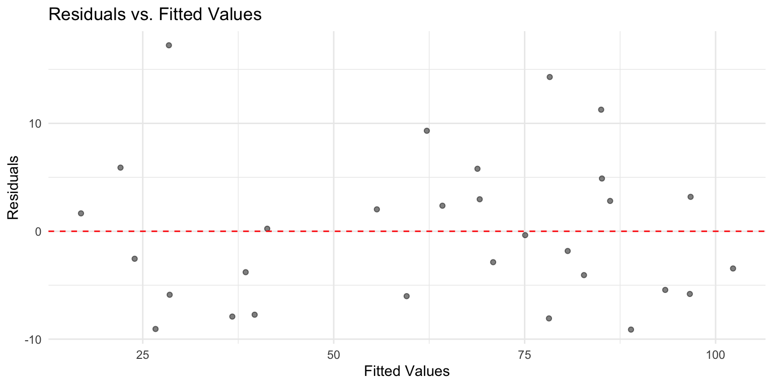
Look for: funnel shapes, increasing/decreasing spread, or other patterns.
What to do about heteroscedasticity?
Several options to address heteroscedasticity:
- Transform the outcome variable (e.g., log transformation)
- Use robust standard errors (also called heteroscedasticity-consistent SEs)
- Use weighted least squares regression
We won’t be covering (2) or (3), but there are R packages for implementing both.
Multicollinearity
Multicollinearity occurs when predictor variables are highly correlated with each other.
- Makes it difficult to isolate the individual effect of each predictor.
- Leads to unstable coefficient estimates with large standard errors.
- Coefficients may have unexpected signs or magnitudes.
- Does NOT affect predictions, but makes interpretation problematic.
Multicollinearity: The core problem
When predictors are highly correlated, the model struggles to determine which predictor is “responsible” for variation in Y.
Consider predicting income from: - Years of education - Number of graduate degrees
- These are highly correlated - more years usually means more degrees.
- The model faces a credit assignment challenge: Is income higher because of years OR degrees?
- Many combinations of coefficients can fit the data equally well.
- Result: Coefficients become unstable and uncertain.
Example: Detecting multicollinearity
Let’s check the correlation between our predictors:
Variance Inflation Factor (VIF)
The VIF quantifies how much the variance of a coefficient is inflated due to multicollinearity.
Seniority Education
1.039324 1.039324 - VIF = 1: No correlation with other predictors
- VIF < 5: Generally acceptable
- VIF > 10: Serious multicollinearity problem
- VIF > 5: Some concern, investigate further
Understanding VIF: The concept
VIF (Variance Inflation Factor) quantifies how much multicollinearity inflates the variance of a coefficient.
From the formula on the previous slide:
\(VIF_j = \frac{1}{1-R^2_j}\)
Where \(R^2_j\) is the R-squared from regressing predictor \(X_j\) on all other predictors.
- Interpretation: “How much is the variance of \(\hat{\beta}_j\) inflated compared to if \(X_j\) were uncorrelated with other predictors?”
- If \(X_j\) is uncorrelated with others: \(R^2_j = 0\) → \(VIF = 1\) (no inflation)
- If \(X_j\) is highly correlated with others: \(R^2_j\) close to 1 → \(VIF\) is large
What to do about multicollinearity?
Several strategies to address multicollinearity:
- Remove one of the correlated predictors
- Combine correlated predictors (e.g., create an index)
- Use principal components analysis (PCA) to create uncorrelated predictors
- Use regularization methods (Ridge, Lasso regression)
- Collect more data with greater variation in predictors
Note
The best solution depends on your research question and theoretical considerations!
Your turn: Diagnostics
Using the mtcars dataset:
- Build a model predicting
mpgfromwt,hp, anddisp - Check for multicollinearity using
cor()andvif() - Create a residual plot to check for heteroscedasticity
- What potential issues do you notice?
Final summary
- Standard errors quantify uncertainty in coefficient estimates
- t-statistics test whether coefficients differ significantly from zero
- Heteroscedasticity (non-constant variance) violates regression assumptions
- Multicollinearity (correlated predictors) inflates standard errors and makes interpretation difficult
- Both issues can be diagnosed and addressed with appropriate techniques
- Always check your model assumptions!
Key takeaways
- Multiple regression allows us to model complex relationships
- Adding interactions captures when one variable’s effect depends on another
- Adjusted \(R^2\) and AIC help compare models with different numbers of predictors
- Understanding SEs helps us assess the reliability of our estimates
- Checking assumptions (homoscedasticity, no multicollinearity) is crucial
- When assumptions are violated, specialized techniques can help
CSS 211 | UC San Diego