Logistic Regression

Goals of the lecture

Classification: dealing with categorical outcomes.
Logistic regression.
- Why not linear regression?
- Generalized linear models (GLMs).
- Odds and log-odds.
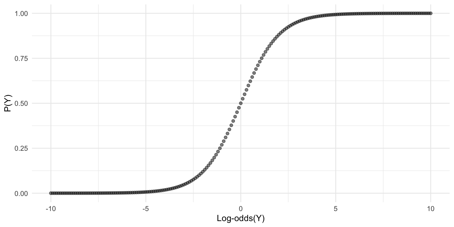
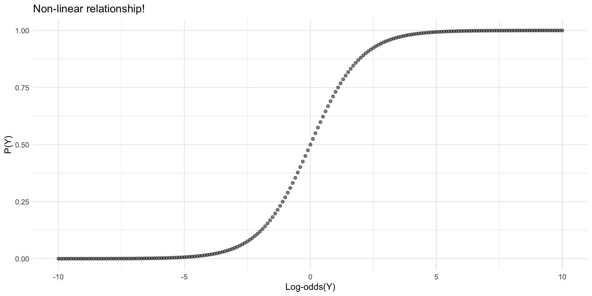
- The logistic function.
Building and interpreting logistic models with glm.

What is classification?

“To classify is human…We sort dirty dishes from clean, white laundry from colorfast, important email to be answered from e-junk…. Any part of the home, school, or workplace reveals some such system of classification.”

— Bowker & Star, 2000

Classification = predicting a categorical response variable using features
Common examples:
- Is an email spam or not spam?
- Is a cell mass cancerous or not cancerous?
- Will this customer buy or not buy?
- Is a credit card transaction fraudulent?
- Is this image a cat, dog, person, or other?

Binary vs. multi-class classification

Binary classification: sorting inputs into one of two labels
- E.g., spam vs. not spam
Multi-class classification: more than two labels
- E.g., face recognition with n possible identities
- E.g., image classification (cat, dog, person, other)
Today: focus on binary classification with logistic regression

Part 1: Foundations of logistic regression

Motivation, log-odds, and the logistic function.

Example dataset: Email spam

### Loading the tidyverse
library(tidyverse)

df_spam = read_csv("https://raw.githubusercontent.com/seantrott/ucsd_css211_datasets/main/main/logistic/spam.csv")
nrow(df_spam)

[1] 3921

Why not linear regression?

spam is coded as 0 (no) or 1 (yes)
Could we treat this as continuous and use linear regression?
Interpret prediction \(\hat{y}\) as probability of outcome?

💭 Check-in

What issues might arise here?

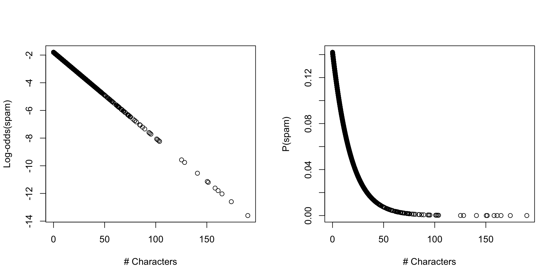
The problem: predictions beyond [0,1]

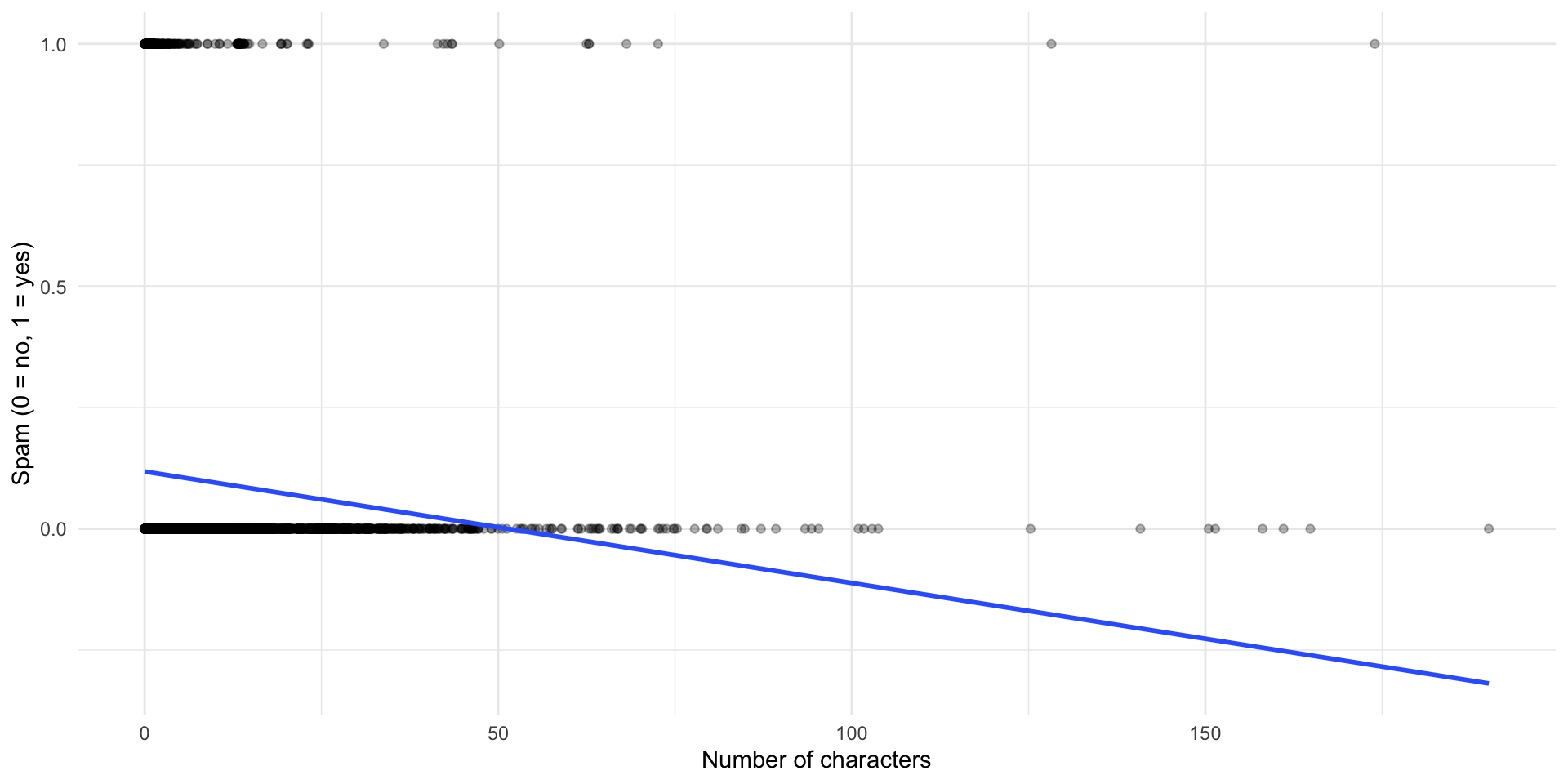
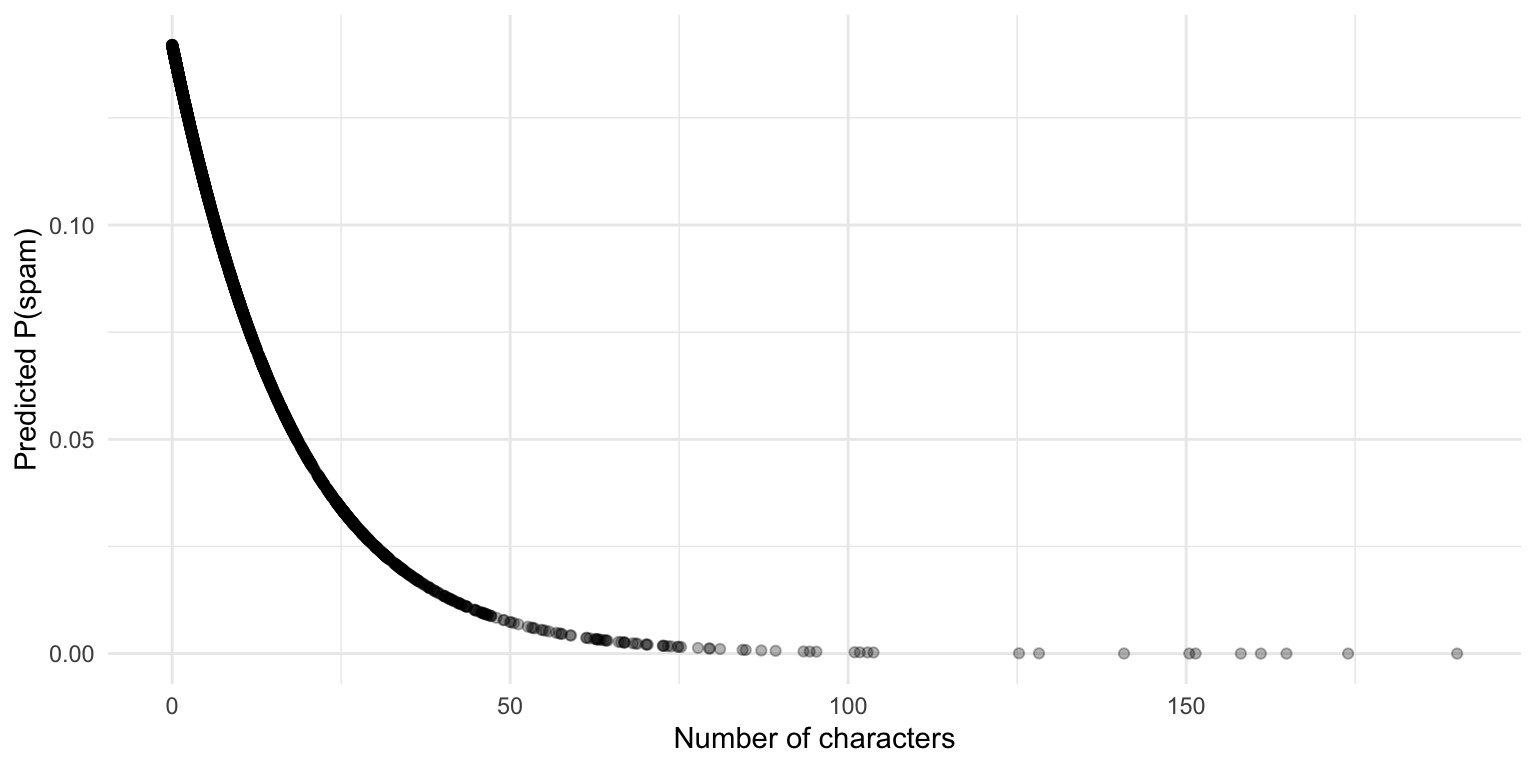
ggplot(df_spam, aes(x = num_char, y = spam)) +
  geom_point(alpha = 0.3) +
  geom_smooth(method = "lm", se = FALSE) +
  labs(x = "Number of characters",
       y = "Spam (0 = no, 1 = yes)") +
  theme_minimal()

Linear model generates predictions outside [0,1], but probability must be bounded!

Framing the problem probabilistically

Treat each outcome as Bernoulli trials: “success” (spam) vs. “failure” (not spam)
Each observation has independent probability of success: \(p\)
On its own: \(p\) = proportion of spam emails
Goal: model \(p\) conditioned on other variables, i.e., \(P(Y = 1 | X)\)

Question: What does \(p\) on its own remind you of from linear regression?

Answer: The intercept-only model (the mean of \(Y\))

Generalized linear models (GLMs)

Generalized linear models (GLMs) are generalizations of linear regression.

Each GLM has:

A probability distribution for the outcome variable
A linear model: \(\beta_0 + \beta_1 X_1 + ... + \beta_k X_k\)
A link function relating the linear model to the outcome

We need a function that links our linear model to a probability score bounded at [0, 1].

Common GLMs

Model name	Distribution	Link function	Use cases	Example
Linear regression	Normal	Identity	Continuous response	Height, price
Logistic regression	Bernoulli/Binomial	Logit	Binary response	Spam, fraud
Poisson regression	Poisson	Log	Count data	# words, # visitors

Today: logistic regression

The logit link function

Logistic regression uses the logit link function:

\[\text{logit}(p) = \log\left(\frac{p}{1-p}\right)\]

Where \(p\) is the probability of some outcome
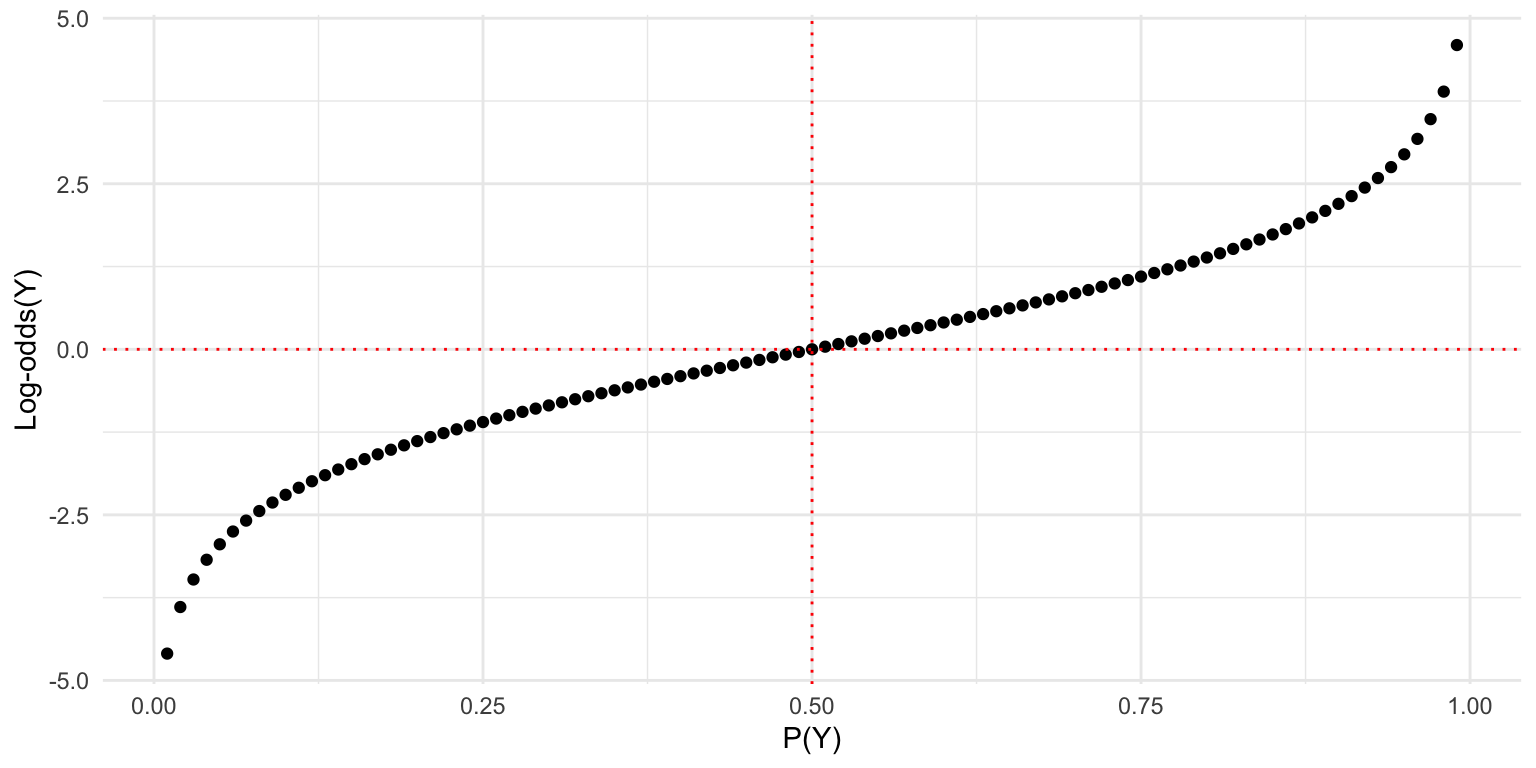
Takes a value between \([0, 1]\) and maps it to \((-\infty, \infty)\)
Also called the log-odds

Introducing the odds

The odds of an event are the ratio of the probability of an event occuring (\(p\)) and the probability of event not occurring (\(1-p\)).

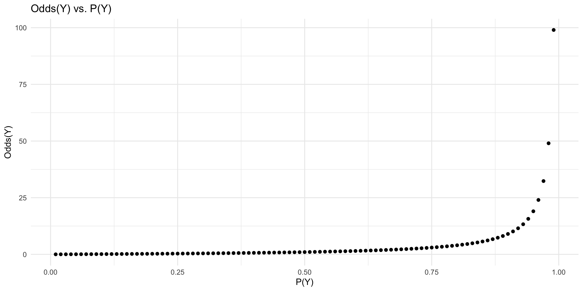
\[\text{Odds}(Y) = \frac{p}{1-p}\]

Unlike \(p\), odds are bounded at \([0, \infty)\)
Odds of 1 means 50/50 chance
Odds > 1 means more likely to occur than not
Odds < 1 means less likely to occur than not

Visualizing odds

p <- seq(0.01, 0.99, 0.01)
odds <- p / (1 - p)

ggplot(data.frame(p, odds), aes(x = p, y = odds)) +
  geom_point() +
  labs(x = "P(Y)", y = "Odds(Y)", 
       title = "Odds(Y) vs. P(Y)") +
  theme_minimal()

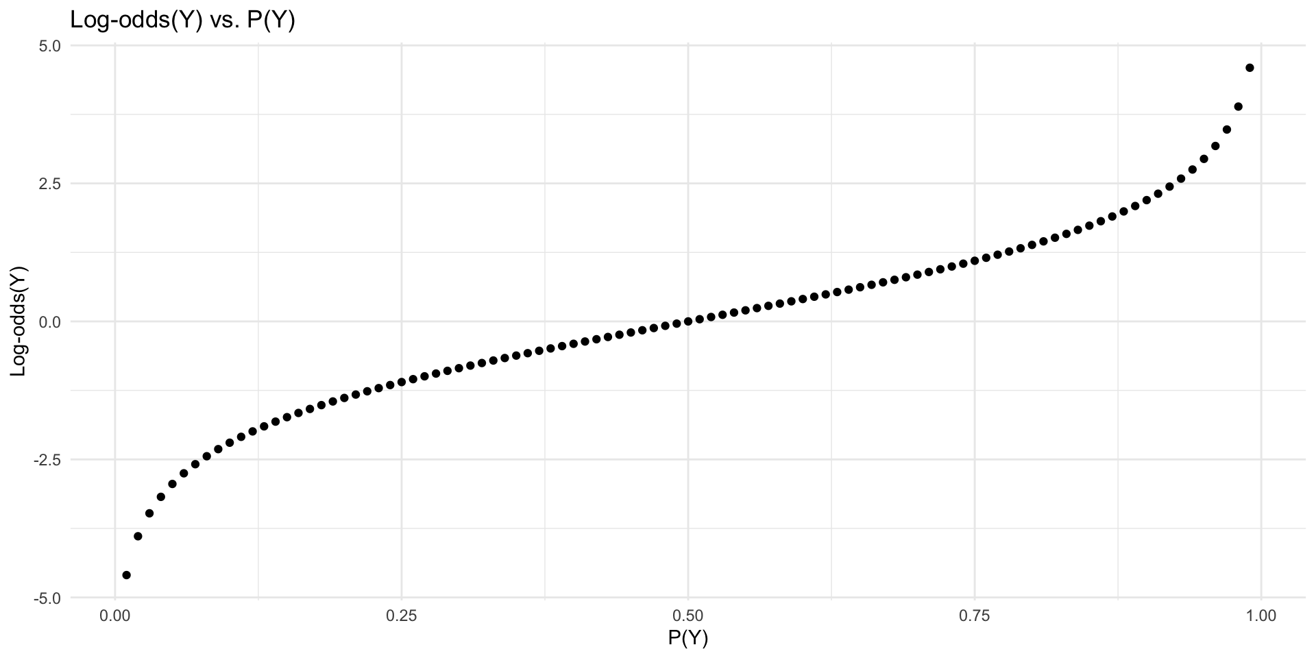
Introducing the log-odds (logit)

The log-odds is the log of the odds (the logit function).

\[\text{logit}(p) = \log\left(\frac{p}{1-p}\right)\]

Unlike \(p\), log-odds are bounded at \((-\infty, \infty)\)
This is what we’ll model linearly!

Visualizing log-odds

log_odds <- log(p / (1 - p))

ggplot(data.frame(p, log_odds), aes(x = p, y = log_odds)) +
  geom_point() +
  labs(x = "P(Y)", y = "Log-odds(Y)", 
       title = "Log-odds(Y) vs. P(Y)") +
  theme_minimal()

Interpreting the sign of log-odds

ggplot(data.frame(p, log_odds), aes(x = p, y = log_odds)) +
  geom_point() +
  geom_vline(xintercept = 0.5, linetype = "dotted", color = "red") +
  geom_hline(yintercept = 0, linetype = "dotted", color = "red") +
  labs(x = "P(Y)", y = "Log-odds(Y)") +
  theme_minimal()

Positive log-odds → \(p > 0.5\)
Negative log-odds → \(p < 0.5\)

The logistic function

The logistic function is the inverse of the logit function.

\[P(Y) = \frac{e^{\text{logit}(p)}}{1 + e^{\text{logit}(p)}}\]

Converts log-odds back to probability
Maps \((-\infty, \infty)\) to \([0, 1]\)
Also called the sigmoid function

Mapping from log-odds to probability

log_odds_range <- seq(-10, 10, 0.1)
p_range <- exp(log_odds_range) / (1 + exp(log_odds_range))
ggplot(data.frame(log_odds_range, p_range), 
       aes(x = log_odds_range, y = p_range)) +
  geom_point(alpha = 0.5) +
  labs(x = "Log-odds(Y)", y = "P(Y)") +
  theme_minimal()

Where does regression come in?

With logistic regression, we learn parameters \(\beta\) for:

\[\log\left(\frac{p}{1-p}\right) = \beta_0 + \beta_1 X_1 + ... + \beta_k X_k\]

Our “dependent variable” is the log-odds (logit) of \(p\)
We learn a linear relationship between \(X\) and the log-odds of our outcome
NOT a linear relationship with probability itself!

Interpreting β: log-odds ~ X is linear

\[\log\left(\frac{p}{1-p}\right) = \beta_0 + \beta_1 X\]

If \(\beta_1 > 0\): For each 1-unit increase in \(X\), log-odds increase by \(\beta_1\)
If \(\beta_1 < 0\): For each 1-unit increase in \(X\), log-odds decrease by \(|\beta_1|\)
Straightforward linear interpretation for log-odds

Interpreting β: P(Y) ~ X is NOT linear

The mapping between log-odds and \(P(Y)\) is not linear.

We cannot interpret coefficients linearly with respect to \(P(Y)\)!

Part 2: Logistic regression in R

Using glm, interpreting logistic models.