Introduction to R

Goals of the lecture

• Brief tooling.
• Why R?
• Introduction to “base R”.
• Brief preview of the tidyverse.

Note

Note that today’s lecture will extend to Friday’s in-class lab slot. Depending on whether we have time on Friday, we can also work on the take-hom lab in Friday’s class.

Tooling (briefly)

One of the most frustrating parts of programming is tooling: getting your computer set up to actually do the stuff you want to learn about.

In this class, we’ll be working with the R programming language using a desktop IDE called RStudio.

• Links to download and install RStudio can be found here.
• Follow the instructions: will include downloading and installing R.
  
• To avoid other tooling headaches, we’ll just be using Canvas for course management.
• We won’t be relying on GitHub, but it’s also very useful and important!

Why R?

There are many different programming languages. Why use R?

• R was specifically designed for data analysis.
  
• R supports a number of open-source packages to make data analysis easier.
  • ggplot, dplyr, lme4.
  • We’ll be learning all about these in the course!
• Other CSS-relevant languages include Python and SQL.
  • Learning R is not incompatible with learning these!

Introduction to “base” R

“Base” R just refers to the set of functions and tools available “out of the box”, without using additional packages like tidyverse.

Base R includes (but is not limited to):

• Basic mechanics like variable assignment.
• Simple functions like plot, as well as core types like vectors.
• Statistical methods like lm and anova (which we’ll discuss later).

Variable assignment

Variables allow us to store information (values, vectors, etc.) so we can use it again later.

Here, we create a variable called account, so we can add to it.

# Our first R variable
account <- 20 ### assign value to variable
account + 25 ### add to variable

[1] 45

Note

You can also use = for assignment, but <- is the R convention. (For most purposes in this course, it shouldn’t matter which you use, and I sometimes mix them up!)

Note💭 Check-in

Try adding different numbers to account. What do you think will happen if you add a string like 'CSS'?

Basic variable types

Each variable has a certain type or class.

You can do different things with different types of variables. For instance, you can’t calculate the mean of multiple characters, but you can for numeric types.

Type	What it is	Example
numeric	Numbers (integers & decimals)	age <- 25, gpa <- 3.7
character	Text strings	name <- "Alice"
logical	TRUE/FALSE values	passed <- TRUE
integer	Whole numbers only	count <- 5L
factor	Categorical data	grade <- factor("A")

Note💭 Check-in

Use the typeof() or class() functions to check the type of different variables or values.

Basic Operations with Numeric Variables

numeric variables allow for a number of arithmetic operations (like a calculator).

# Creating numeric variables
my_var <- 5


my_var + 1 ### Addition

[1] 6

my_var * 2 ### Multiplication

[1] 10

my_var / 2 ### Division

[1] 2.5

my_var ** 2 ### Exponentiation

[1] 25

Vectors: Building Blocks of R

A vector is a collection of elements with the same class.

Vectors can be created with the c(...) function.

# Creating vector
my_vector <- c(25, 30, 32)
print(my_vector)

[1] 25 30 32

print(my_vector[1])

[1] 25

Note💭 Check-in

Create your own vector, this time with character types in it. Try indexing into different parts of the vector.

Working with vectors

Like scalars, numeric vectors can be manipulated mathematically.

my_vector + 1 ### add 1 to each element

[1] 26 31 33

my_vector * 5 ### Multiply each element by 5

[1] 125 150 160

my_vector + c(1, 2, 3) ### Add vector to another vector

[1] 26 32 35

Note💭 Check-in

What do you think will happen if you try to add two vectors of different lengths?

Functions

A function implements some operation; you can think of it as a verb applied to some input.

In CSS, you’ll often be using functions to summarize your data (like a vector).

# Creating vector
heights <- c(60, 65, 62, 70, 72, 73)

mean(heights)

[1] 67

median(heights)

[1] 67.5

Note💭 Check-in

Create a vector containing possible incomes; then create the mean and median of this vector.

Creating vectors from distributions (pt. 1)

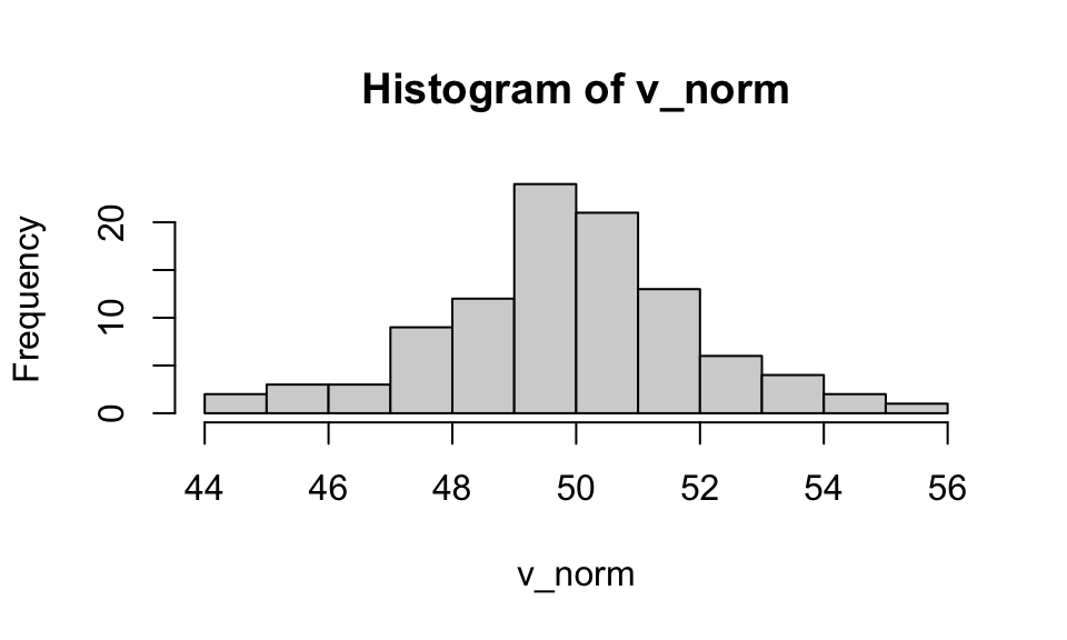
In addition to creating vectors by hand, we can use functions to create random vectors by sampling from some distribution, e.g., a normal distribution (rnorm(x, mean, sd)).

# Creating vector
v_norm = rnorm(100, mean = 50, sd = 2)
hist(v_norm)

Note💭 Check-in

Try changing the different parameters of rnorm and then plotting the resulting vector again using hist. What do you notice about changing the mean or sd?

Creating vectors from distributions (pt. 2)

There are also many types of distributions beyond normal distributions.

• Uniform distributions: use runif.
• Binomial distributions: use rbinom.
• Poisson distributions: use rpois.
• Sampling from these distributions (and visualizing them) is a helpful way to learn about different statistical distributions.

Note💭 Check-in

Create a uniform distribution with runif with 100 values ranging from 2 to 3. If you’re not sure how to do this, use ?runif to learn more about the function.

Interim summary

So far, we’ve covered a number of core topics in base R.

• Assigning and working with variables.
• Different types of variables.
• Applying functions to variables.
• Creating vectors and visualizing them with hist.
• Sampling from statistical distribution.

Note💭 Check-in

Any questions before we move on to creating dataframes and other kinds of plots?

Dataframes

The data.frame class is a “tightly coupled collection of variables”; it’s also a fundamental data structure in R.

• Like a matrix, but with labeled columns of the same length.
• Each column corresponds to a vector of values (numbers, characters, etc.).
• Supports many useful operations.
• Analogous to pandas.DataFrame in Python!

Note

Note that once we move to the tidyverse, we’ll be working with tibbles, which are basically like a data.frame.

Creating a data.frame

• A data.frame can be created using the data.frame function.
• Pass in labeled vectors of the same length.

df_example = data.frame(hours_studied = c(0, 2, 2, 3, 5, 8), test_score = c(70, 85, 89, 89, 94, 95))
head(df_example, 2)

  hours_studied test_score
1             0         70
2             2         85

Note💭 Check-in

Try creating your own data.frame with custom columns. For example, one column could be movie_title and another could be your rating of that movie. Make sure the columns are the same length!

Exploring a data.frame

We can use functions like nrow, head, and colnames to learn about our data.frame.

print(nrow(df_example)) ### How many rows?

[1] 6

print(colnames(df_example)) ### Column names

[1] "hours_studied" "test_score"   

print(head(df_example, 2)) ### First two rows

  hours_studied test_score
1             0         70
2             2         85

print(str(df_example)) ### Structure of data

'data.frame':   6 obs. of  2 variables:
 $ hours_studied: num  0 2 2 3 5 8
 $ test_score   : num  70 85 89 89 94 95
NULL

print(summary(df_example)) ### Summary of each column

 hours_studied     test_score   
 Min.   :0.000   Min.   :70.00  
 1st Qu.:2.000   1st Qu.:86.00  
 Median :2.500   Median :89.00  
 Mean   :3.333   Mean   :87.00  
 3rd Qu.:4.500   3rd Qu.:92.75  
 Max.   :8.000   Max.   :95.00  

Accessing individual columns

You can access individual columns using the dataframe$column_name syntax.

df_example$hours_studied ### Get vector

[1] 0 2 2 3 5 8

summary(df_example$hours_studied) ### Get summary of vector

   Min. 1st Qu.  Median    Mean 3rd Qu.    Max. 
  0.000   2.000   2.500   3.333   4.500   8.000 

Filtering a data.frame

In base R, you can filter a data.frame using the df[CONDITION] syntax, where CONDITION corresponds to a logical statement.

df_example[df_example$hours_studied > 2, ]

  hours_studied test_score
4             3         89
5             5         94
6             8         95

Note

In the tidyverse, we can use the handy filter function.

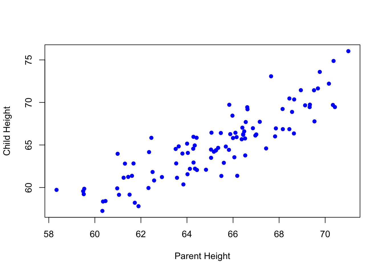
Simple bivariate plots

Once you have multiple vectors, you can plot the relationship between them, e.g., using a simple scatterplot.

plot(df_example$hours_studied, 
     df_example$test_score,
     xlab = "Hours Studied", 
     ylab = "Test Score",
     pch = 16, # Filled circles
     col = "blue")

Calculating correlations

You can also quantify the relationship between variables, e.g., using a Pearson’s r correlation coefficient.

cor.test(df_example$hours_studied, df_example$test_score)

    Pearson's product-moment correlation

data:  df_example$hours_studied and df_example$test_score
t = 2.8958, df = 4, p-value = 0.0443
alternative hypothesis: true correlation is not equal to 0
95 percent confidence interval:
 0.03391115 0.97998161
sample estimates:
      cor 
0.8228274 

Working with missing data

Real data often contains missing values. R represents these as NA (Not Available). We’ll discuss these in more detail next week, but here’s a preview:

# Vector with missing data
survey_responses <- c(85, 92, NA, 78, NA, 88)
mean(survey_responses)                    # Returns NA!

[1] NA

mean(survey_responses, na.rm = TRUE)      # Remove NAs first: 85.75

[1] 85.75

Working with missing data (pt. 2)

You can remove missing data by filtering the data.frame, using the syntax below and the is.na condition.

# Vector with missing data
survey_responses[is.na(survey_responses) == FALSE]

[1] 85 92 78 88

Putting it together: simulating data

So far, we’ve discussed a number of useful concepts in R:

• Working with vectors.
• Simulating random distributions using rnorm.
• Creating data.frame objects and plotting or analyzing them.

Note💭 Check-in

Now, let’s simulate data.

• First, use rnorm to create a random normal distribution of parent_heights (use parameters that seem reasonable to you).
• Then, create a second variable called child_heights that’s related to parent_heights, ideally with some random error added. (Hint: Think about how a regression line works.).
• Put these variables in a data.frame.
• Finally, plot the relationship between those variables and calculate the correlation.

Simulating data

parent_heights = rnorm(100, 65, 3)
child_heights = parent_heights + rnorm(100, 0, 2)
df_heights = data.frame(parent_heights, child_heights)

plot(df_heights$parent_heights, 
     df_heights$child_heights,
     xlab = "Parent Height", 
     ylab = "Child Height",
     pch = 16, # Filled circles
     col = "blue")

cor(df_heights$parent_heights, df_heights$child_heights)

[1] 0.871996

A conceptual preview of the tidyverse

Next week, we’ll discuss the tidyverse: a set of packages and functions developed to make data analysis and visualization in R easier.

This includes (but is not limited to):

• Functions for transforming data, e.g., filter or mutate.
• Functions for merging data, like left_join or inner_join.
• Functions for visualizing data, like ggplot.

Lecture wrap-up

This course is not primarily about programming in R, but programming in R is a foundational skill for other parts of this course.

This lecture (and accompanying lab) is intended to give you more comfort with the following concepts:

• Working with variables and different types of data.
• Creating and working with vectors.
  
• Simple plotting.
• Working with data.frame objects.