Model comparison: the logic of likelihood-ratio tests.
glmer: generalized linear mixed models.
Best practices.
Load libraries
### Loading the tidyverselibrary(tidyverse)
── Attaching core tidyverse packages ──────────────────────── tidyverse 2.0.0 ──
✔ dplyr     1.1.4     ✔ readr     2.1.5
✔ forcats   1.0.0     ✔ stringr   1.5.1
✔ ggplot2   3.5.2     ✔ tibble    3.2.1
✔ lubridate 1.9.4     ✔ tidyr     1.3.1
✔ purrr     1.0.4
── Conflicts ────────────────────────────────────────── tidyverse_conflicts() ──
✖ dplyr::filter() masks stats::filter()
✖ dplyr::lag()    masks stats::lag()
ℹ Use the conflicted package (<http://conflicted.r-lib.org/>) to force all conflicts to become errors
### Loading lme4library(lme4)
Loading required package: Matrix

Attaching package: 'Matrix'

The following objects are masked from 'package:tidyr':

    expand, pack, unpack
Part 1: Independence
The independence assumption; why it matters; examples of non-independence.
What is independence?
Independence means that each observation in your dataset is generated by a separate, unrelated causal process.
When you flip a coin, each flip is independent of the others
The outcome of flip #1 doesn’t influence flip #2
No hidden factors connect multiple observations
Each data point provides new information
Independence is a fundamental assumption of many statistical tests. When we assume independence, we’re saying that knowing the value of one observation tells us nothing about another observation beyond what our model predicts.
Why does independence matter?
Standard statistical methods (t-tests, OLS regression, ANOVA) assume independence.
When this assumption is violated:
Standard errors are underestimated
Confidence intervals are too narrow
p-values are too small (inflated Type I error)
Your conclusions may be wrong!
The problem: Treating non-independent observations as independent makes you overconfident in your results.
Example: Independent data
You test whether a new drug increases happiness:
100 people receive the drug
100 people receive a placebo
Each person provides one happiness rating (1-7 scale)
You compare the two groups with a t-test
✓ Independence is reasonable here
Each person contributes exactly one data point.
Another independent example
You test whether people respond differently to metaphor type A vs. B:
200 participants, randomly assigned to condition A or B
Each participant sees one item
Between-subjects design with one item per person
Compare responses with OLS regression
✓ Independence is reasonable here
No repeated measures, no item effects to worry about.
Visualizing independent data
Each observation is independent—no nesting structure.
Analyzing independent data
simple_model =lm(data = df, value ~ group)summary(simple_model)$coefficients
             Estimate Std. Error   t value      Pr(>|t|)
(Intercept) 726.87939   1.418843 512.30416 4.019115e-311
groupB      -21.80864   2.006548 -10.86874  7.022045e-22
Interpretation: - Intercept (groupA) = 726.88 (mean of group A) - groupB coefficient = -21.81 (difference from A) - Group B is about 20 units lower than Group A
When independence fails
Non-independence occurs when different observations are systematically related, i.e., they were produced by the same generative process.
Common sources of non-independence in behavioral research:
Repeated measures: Same participant tested multiple times
Nested data: Students within classrooms within schools
Stimulus items: Same stimuli shown to multiple participants
Time series: Measurements over time from same units
Clustered designs: Participants recruited from same communities
Example: The sleep study
The sleepstudy dataset tracks reaction times in 18 subjects over subsequent days of sleep deprivation:
Based on the structure of this study, what might be a source of non-independence?
Naive analysis (wrong!)
Let’s pretend we don’t know about the nested structure:
sleepstudy %>%ggplot(aes(x = Days, y = Reaction)) +geom_point(alpha =0.5) +geom_smooth(method ="lm", color ="red") +labs(title ="Naive analysis: treating all 180 observations as independent") +theme_minimal(base_size =14)
`geom_smooth()` using formula = 'y ~ x'
Note💭 Check-in
What’s not pictured here?
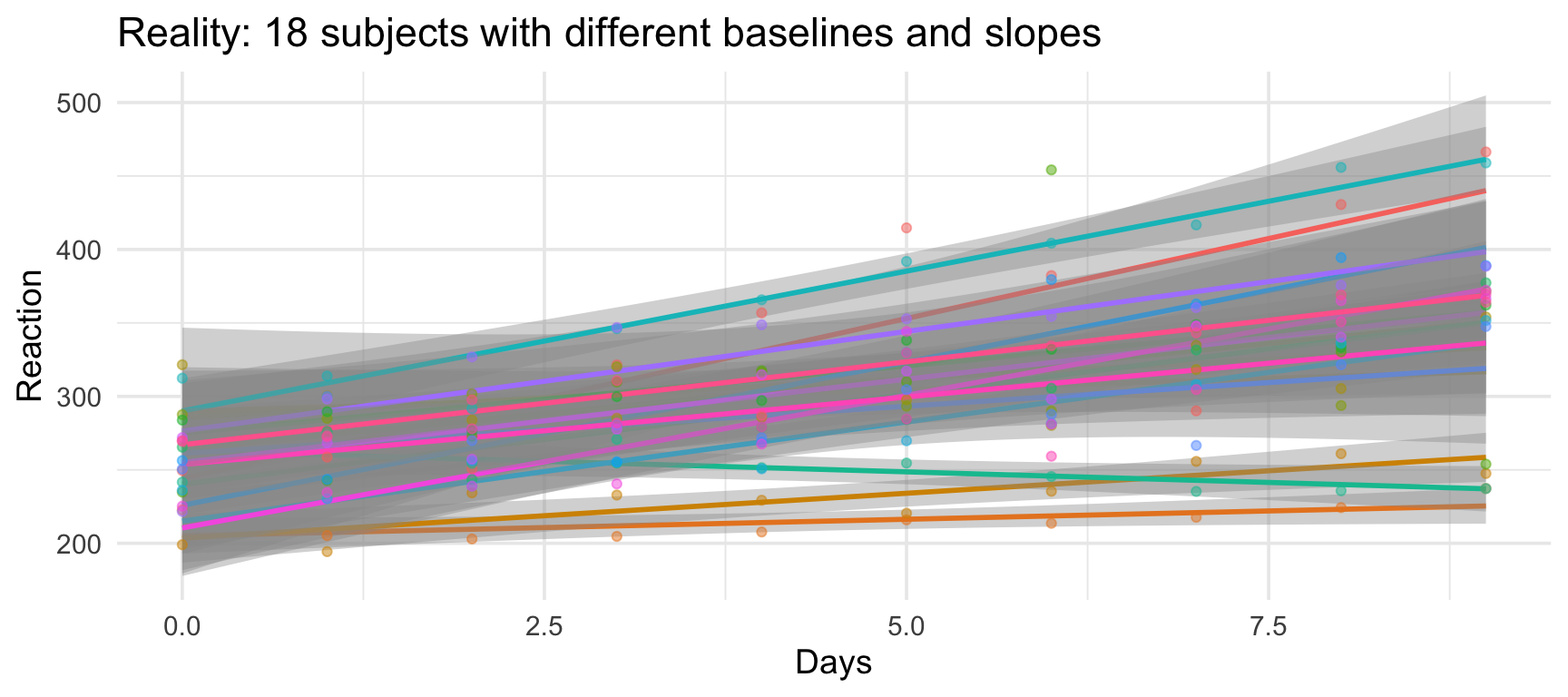
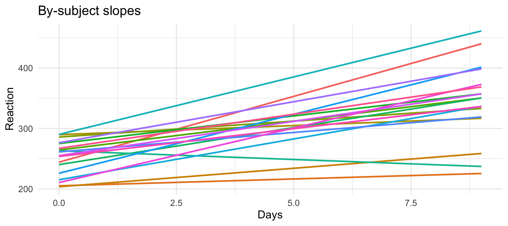
The real structure
`geom_smooth()` using formula = 'y ~ x'
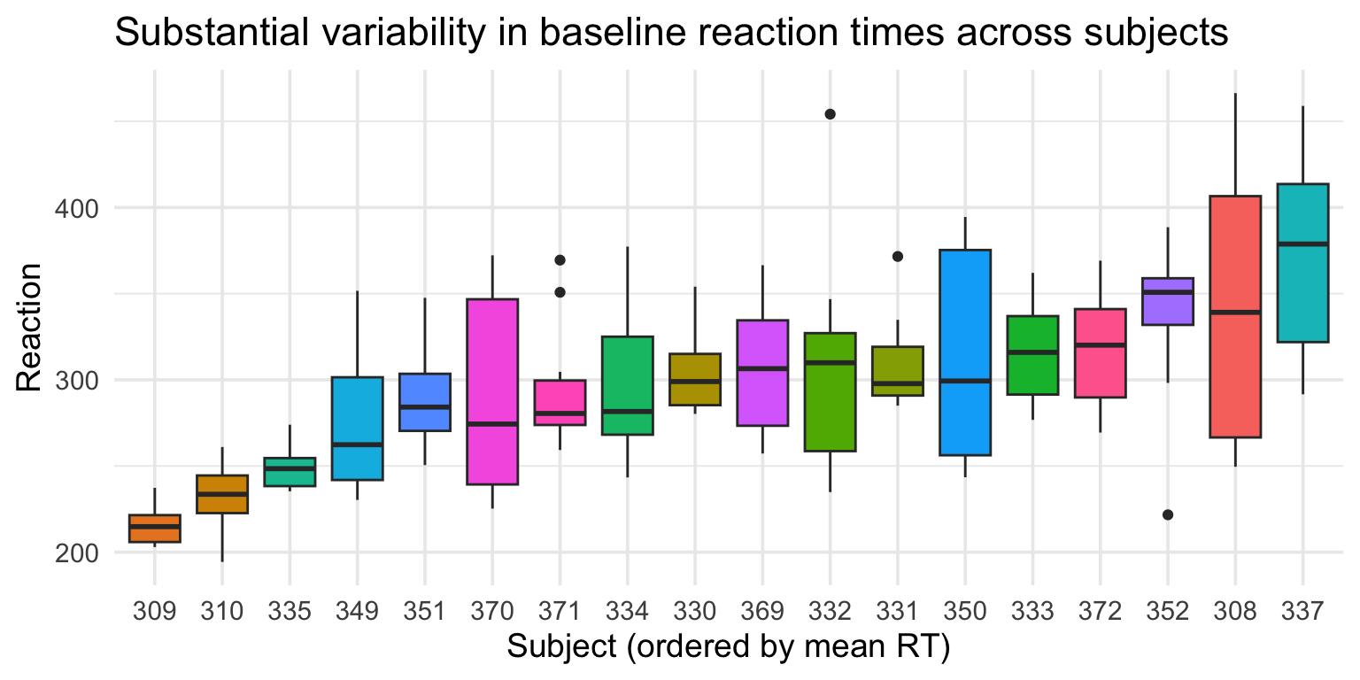
Subjects differ in:
Overall reaction time (baseline speed)
Effect of sleep deprivation (some are more resilient)
Subject-level variability
Some subjects are consistently faster; others are consistently slower.
Two types of nested variance
Random intercepts: Subjects differ in their average reaction time
Some people are just faster/slower overall
Even with no sleep deprivation!
Random slopes: Subjects differ in how much sleep deprivation affects them
Some people are resilient (shallow slope)
Others deteriorate quickly (steep slope)
Mixed effects models let us account for both types of variance.
Part 2: Introduction to mixed effects models
Fixed vs. random effects; random intercepts; random slopes.
What are mixed effects models?
Mixed effects models combine:
Fixed effects: Variables we care about (e.g., experimental conditions)
These are your hypotheses!
Estimated with specific coefficient values
Random effects: Grouping variables that create non-independence
Sources of variability we need to control for
Allow intercepts/slopes to vary by group
Estimated as distributions (variance parameters)
Goal: Get better estimates of fixed effects by accounting for nested structure.
Fixed vs. random effects
Determining which factors to include as fixed vs. random effects is not always straightforward. Here’s a rough guide, but we’ll discuss it again later too:
How do you decide?
Fixed effects:
Variables you’re theoretically interested in
Want to estimate specific coefficient values
Often experimental manipulations
Examples: treatment condition, time, drug dosage
Random effects:
Grouping/clustering variables
Want to account for variance, not estimate specific values
Usually sampling from larger population
Examples: participant ID, item ID, school, lab
The mixed model formula
Standard regression:
\[Y = \beta_0 + \beta_1 X + \epsilon\]
Mixed effects model with random intercepts:
\[Y = (\beta_0 + u_0) + \beta_1 X + \epsilon\]
Where:
\(\beta_0\) = overall intercept (fixed effect)
\(u_0\) = subject-specific deviation from overall intercept (random effect)
\(\beta_1\) = fixed effect of X
\(\epsilon\) = residual error
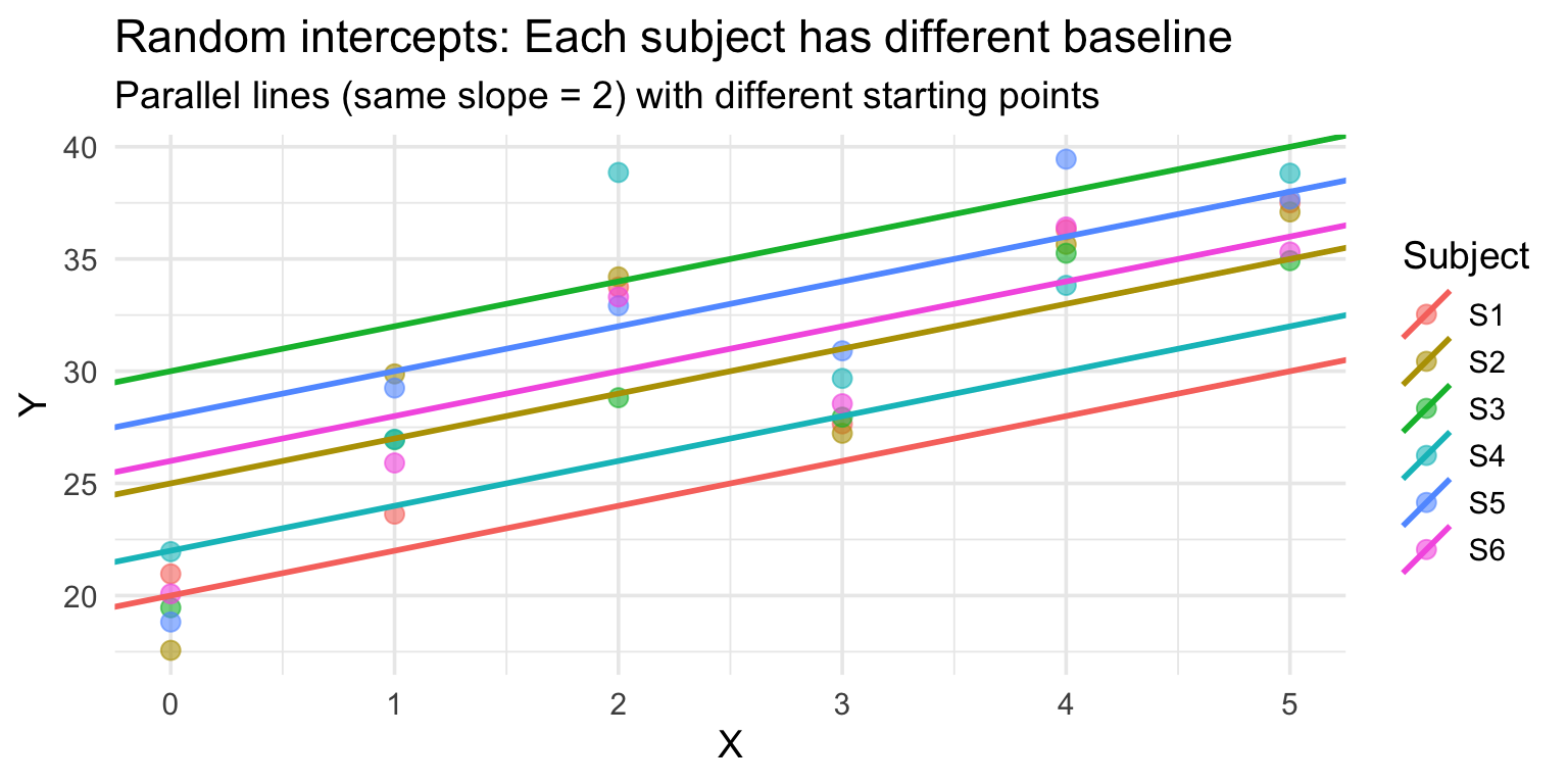
Random intercepts: Intuition
Random intercepts allow each group (e.g., subject) to have its own baseline:
Same slope, different intercepts.
Random intercepts: R syntax
Basic model with random intercepts:
model_intercepts <-lmer(Reaction ~ Days + (1| Subject), data = sleepstudy)
Breaking down the syntax:
Reaction ~ Days: Fixed effect of Days on Reaction
(1 | Subject): Random intercept for each Subject
1 = intercept
| = “grouped by”
Subject = grouping variable
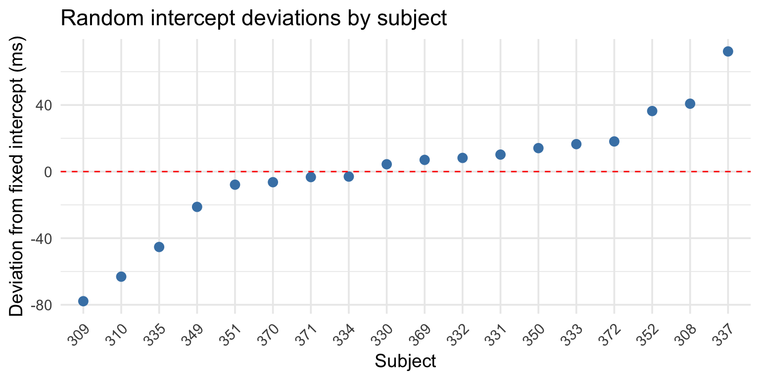
Extracting random intercepts
After fitting the model, you can extract the random effects:
# Extract random interceptsrandom_int <-ranef(model_intercepts)$Subjecthead(random_int, 4)
Subject 308’s RT increases by ~19.67 ms per day (vs. population average of ~10.47 ms).
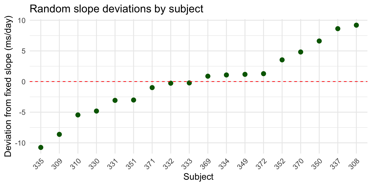
Visualizing random slopes
# Create dataframe of random effectsslopes_df <-ranef(model_slopes)$Subject %>%rownames_to_column("Subject") %>%rename(intercept_dev =`(Intercept)`, slope_dev = Days)ggplot(slopes_df, aes(x =reorder(Subject, slope_dev), y = slope_dev)) +geom_point(size =3, color ="darkgreen") +geom_hline(yintercept =0, linetype ="dashed", color ="red") +labs(title ="Random slope deviations by subject",x ="Subject", y ="Deviation from fixed slope (ms/day)") +theme_minimal(base_size =14) +theme(axis.text.x =element_text(angle =45, hjust =1))
Why random slopes matter
Without random slopes: - Assumes the effect is the same for everyone - Underestimates uncertainty in the fixed effect - Can lead to false positives
With random slopes: - Acknowledges that effects vary across individuals - Provides more conservative (realistic) estimates - Better generalization to new subjects
Rule of thumb: If a variable varies within your grouping variable, include it as a random slope.
Multiple random effects
You can include multiple sources of random effects:
# Random effects for both subjects and itemsmodel <-lmer(RT ~ Condition + (1+ Condition | Subject) + (1+ Condition | Item),data = mydata)
Common in psycholinguistics: - Random effects for subjects (people vary) - Random effects for items (stimuli vary) - Called “crossed random effects”
Conceptual summary
Mixed effects models help when:
You have repeated measures
You have nested/hierarchical structure
You want to generalize beyond your specific sample
Key components:.
Fixed effects: Your hypotheses.
Random intercepts: Group-level baseline differences
Random slopes: Group-level differences in effects.
Part 3: Using lme4
Building and evaluating models; model comparisons; best practices and common issues.
The lme4 package
Most common R package for mixed models:
library(lme4)
Main functions: - lmer(): Linear mixed effects models - glmer(): Generalized linear mixed models (logistic, Poisson, etc.)
Building your first model
Let’s fit a model with random intercepts only:
model_intercepts <-lmer(Reaction ~ Days + (1| Subject),data = sleepstudy,REML =FALSE)
Note:REML = FALSE uses maximum likelihood estimation, which we need for model comparison.
Viewing model output
summary(model_intercepts)
Linear mixed model fit by maximum likelihood ['lmerMod']
Formula: Reaction ~ Days + (1 | Subject)
Data: sleepstudy
AIC BIC logLik -2*log(L) df.resid
1802.1 1814.9 -897.0 1794.1 176
Scaled residuals:
Min 1Q Median 3Q Max
-3.2347 -0.5544 0.0155 0.5257 4.2648
Random effects:
Groups Name Variance Std.Dev.
Subject (Intercept) 1296.9 36.01
Residual 954.5 30.90
Number of obs: 180, groups: Subject, 18
Fixed effects:
Estimate Std. Error t value
(Intercept) 251.4051 9.5062 26.45
Days 10.4673 0.8017 13.06
Correlation of Fixed Effects:
(Intr)
Days -0.380
Adding random slopes
Now let’s add random slopes for the Days effect:
model_full <-lmer(Reaction ~ Days + (1+ Days | Subject),data = sleepstudy,REML =FALSE)
This allows both the intercept AND the slope to vary by subject.
Comparing the models
summary(model_full)
Linear mixed model fit by maximum likelihood  ['lmerMod']
Formula: Reaction ~ Days + (1 + Days | Subject)
   Data: sleepstudy

      AIC       BIC    logLik -2*log(L)  df.resid
   1763.9    1783.1    -876.0    1751.9       174

Scaled residuals:
    Min      1Q  Median      3Q     Max
-3.9416 -0.4656  0.0289  0.4636  5.1793

Random effects:
 Groups   Name        Variance Std.Dev. Corr
 Subject  (Intercept) 565.48   23.780
          Days         32.68    5.717   0.08
 Residual             654.95   25.592
Number of obs: 180, groups:  Subject, 18

Fixed effects:
            Estimate Std. Error t value
(Intercept)  251.405      6.632  37.907
Days          10.467      1.502   6.968

Correlation of Fixed Effects:
     (Intr)
Days -0.138
Model comparison: The logic
The likelihood of a model refers to the probability of the observed data under that model’s parameter estimates.
Question: Does adding variable \(X\) improve the model over a model without \(X\)?
Approach: Likelihood ratio test (LRT)
Compare log-likelihood of two nested models
Model with more parameters should fit better
But: is the improvement “worth it”?
Test statistic: \(\chi^2 = -2(LL_{reduced} - LL_{full})\)
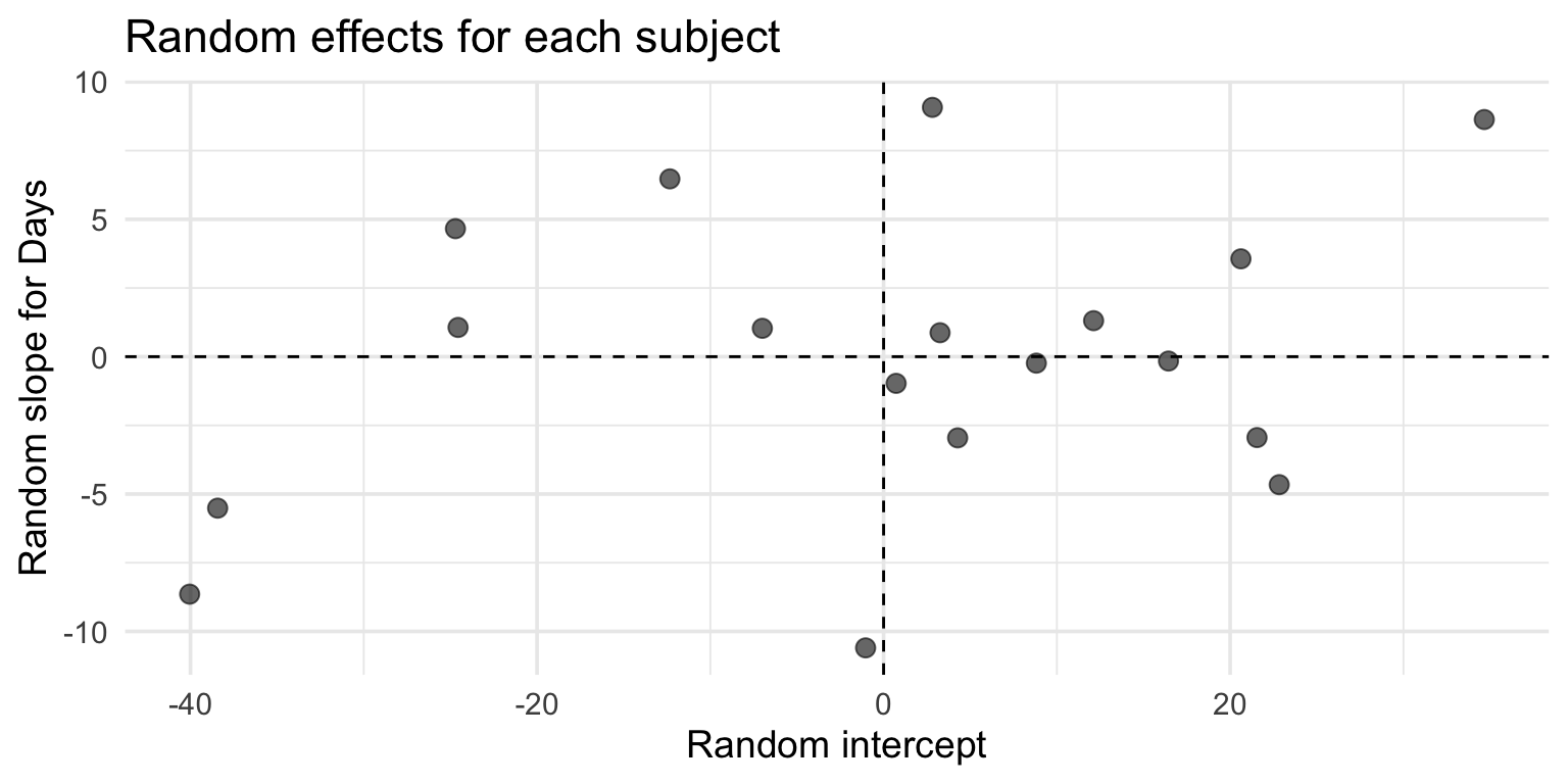
ranef_df <-ranef(model_full)$Subject %>%rownames_to_column("Subject")ggplot(ranef_df, aes(x =`(Intercept)`, y = Days)) +geom_point(size =3, alpha =0.6) +geom_hline(yintercept =0, linetype ="dashed") +geom_vline(xintercept =0, linetype ="dashed") +labs(title ="Random effects for each subject",x ="Random intercept", y ="Random slope for Days") +theme_minimal(base_size =14)
Generalized linear mixed models
A generalized linear mixed model (GLMM) is a general framework for fitting regression models with various link functions (e.g., logit) and random effects.
We’ve already discussed GLMs (glm) and logistic regression.
A GLMM is just a way to add random effects structure to a GLM.
glmer is to glm as lmer is to lm.
Example: Binary outcomes
Scenario: Testing accuracy on a memory task
Each participant completes multiple trials
Each trial is coded as correct (1) or incorrect (0)
We want to know if reaction time predicts accuracy
# Ignoring nested structurenaive_glm <-glm(Correct ~ RT, data = binary_data, family = binomial)summary(naive_glm)$coefficients
                Estimate  Std. Error    z value     Pr(>|z|)
(Intercept) -4.333121392 1.267280721 -3.4192277 0.0006279914
RT           0.001789766 0.002405329  0.7440834 0.4568259948
Problem: This ignores that we have 30 trials per subject! Standard errors will be too small.
Using glmer()
Add random effects for subjects:
# With random interceptsglmm_model <-glmer(Correct ~ RT + (1| Subject),data = binary_data,family =binomial(link ="logit"))
boundary (singular) fit: see help('isSingular')
summary(glmm_model)
Generalized linear mixed model fit by maximum likelihood (Laplace
  Approximation) [glmerMod]
 Family: binomial  ( logit )
Formula: Correct ~ RT + (1 | Subject)
   Data: binary_data

      AIC       BIC    logLik -2*log(L)  df.resid
    174.0     187.2     -84.0     168.0       597

Scaled residuals:
    Min      1Q  Median      3Q     Max
-0.2395 -0.1897 -0.1784 -0.1685  6.4595

Random effects:
 Groups  Name        Variance Std.Dev.
 Subject (Intercept) 0        0
Number of obs: 600, groups:  Subject, 20

Fixed effects:
             Estimate Std. Error z value Pr(>|z|)
(Intercept) -4.333121   1.277856  -3.391 0.000697 ***
RT           0.001790   0.002425   0.738 0.460513
---
Signif. codes:  0 '***' 0.001 '**' 0.01 '*' 0.05 '.' 0.1 ' ' 1

Correlation of Fixed Effects:
   (Intr)
RT -0.983
optimizer (Nelder_Mead) convergence code: 0 (OK)
boundary (singular) fit: see help('isSingular')
Syntax breakdown: - Correct ~ RT: Fixed effect of RT on accuracy - (1 | Subject): Random intercept for each subject - family = binomial(link = "logit"): Logistic regression
Interpreting GLMM output
summary(glmm_model)
Generalized linear mixed model fit by maximum likelihood (Laplace
  Approximation) [glmerMod]
 Family: binomial  ( logit )
Formula: Correct ~ RT + (1 | Subject)
   Data: binary_data

      AIC       BIC    logLik -2*log(L)  df.resid
    174.0     187.2     -84.0     168.0       597

Scaled residuals:
    Min      1Q  Median      3Q     Max
-0.2395 -0.1897 -0.1784 -0.1685  6.4595

Random effects:
 Groups  Name        Variance Std.Dev.
 Subject (Intercept) 0        0
Number of obs: 600, groups:  Subject, 20

Fixed effects:
             Estimate Std. Error z value Pr(>|z|)
(Intercept) -4.333121   1.277856  -3.391 0.000697 ***
RT           0.001790   0.002425   0.738 0.460513
---
Signif. codes:  0 '***' 0.001 '**' 0.01 '*' 0.05 '.' 0.1 ' ' 1

Correlation of Fixed Effects:
   (Intr)
RT -0.983
optimizer (Nelder_Mead) convergence code: 0 (OK)
boundary (singular) fit: see help('isSingular')
Example: Binary outcomes
Scenario: Testing accuracy on a memory task
Each participant completes multiple trials
Each trial is coded as correct (1) or incorrect (0)
We want to know if reaction time predicts accuracy
Part 4: Best practices
Choosing random effects; dealing with convergence warnings; reporting results.
Common questions
Mixed effects models can get complex pretty quickly. Researchers end up running into a number of common questions:
Which effects should be random and which should be fixed?
How many random effects should I specify? Just random intercepts? Random slopes?
What happens if my model doesn’t “converge”?
How do I report my results?
We’ll tackle each of these one by one.
Fixed vs. random?
Selecting fixed vs. random effects can be challenging. There’s not even universal consensus on the best way to do this!
Some ways to think about it:
In terms of sampling: Fixed effects exhaust the theoretical population (e.g., condition 1 vs. condition 2), and random effects are just a sample (e.g., of participants).
In terms of estimation process: Fixed effects are estimated using maximum likelihood estimation, and random effects are estimated with shrinkage.
In terms of interest: Fixed effects are what you’re interested in, and random effects are what you want to control for.
How many random effects to include? (1)
Barr et al. (2013): “Keep it maximal”
Include the most complex random effects structure justified by your design
Include random slopes for within-unit variables
This reduces Type I error and improves generalizability
Example:
# Maximal model for 2x2 design with subjects and itemslmer(RT ~ Condition1 * Condition2 + (1+ Condition1 * Condition2 | Subject) + (1+ Condition1 * Condition2 | Item),data = mydata)
How many random effects to include? (2)
Bates et al. (2015): “Parsimonious mixed models”
Maximal models often fail to converge or produce singular fits (coming up!)
Start with maximal model, then simplify if necessary
Remove random effect correlations first, then non-significant random slopes
Balance between Type I error control and model stability
Computational issues: Model is too complex for data
Dealing with convergence issues
Step 1: Check your data - Are there enough observations per group? - Any extreme outliers?
Step 2: Rescale continuous predictors
data$Days_scaled <-scale(data$Days)
Step 3: Try different optimizer
lmer(Y ~ X + (1+ X | Subject),control =lmerControl(optimizer ="bobyqa"))
Simplifying random effects
Step 4: Simplify random effects structure
Start by removing correlations between random effects:
# Remove correlation between intercept and slopelmer(Reaction ~ Days + (1| Subject) + (0+ Days | Subject))
Step 5: Remove random slopes if necessary
Use model comparison to determine which random effects are necessary (Bates et al., 2015).
Reporting your results
Template for reporting:
We fit a linear mixed effects model predicting reaction time from days of sleep deprivation. The model included random intercepts and random slopes for days grouped by subject. Sleep deprivation significantly increased reaction time (β = 10.47, SE = 1.55), with each additional day of deprivation associated with an ~10.5 ms increase in RT. A likelihood ratio test confirmed that including days as a fixed effect significantly improved model fit, χ²(1) = 45.85, p < 0.001.