Linear regression in R

Goals of the lecture

Foundations of statistical modeling.
Basic goals and assumptions of univariate linear regression.
- Measuring error.
Linear regression in R with lm.
- Interpreting lm model outputs: coefficients, p-values, and \(R^2\).

### Loading the tidyverse
library(tidyverse)

── Attaching core tidyverse packages ──────────────────────── tidyverse 2.0.0 ──
✔ dplyr     1.1.4     ✔ readr     2.1.5
✔ forcats   1.0.0     ✔ stringr   1.5.1
✔ ggplot2   3.5.2     ✔ tibble    3.2.1
✔ lubridate 1.9.4     ✔ tidyr     1.3.1
✔ purrr     1.0.4     
── Conflicts ────────────────────────────────────────── tidyverse_conflicts() ──
✖ dplyr::filter() masks stats::filter()
✖ dplyr::lag()    masks stats::lag()
ℹ Use the conflicted package (<http://conflicted.r-lib.org/>) to force all conflicts to become errors

library(broom)

Part 1: Modeling

What are “models”, and why should we build them?

From descriptions to models

A statistical model is a mathematical model representing a data-generating process.

So far, we’ve focused on describing and visualizing data.
But often, we want to model our data.
- Typically involves learning some function mapping \(X\) to \(Y\).
All models are wrong, but some are useful.

Why models?

Statistical models help us understand our data, and also predict new data.

Prediction: Try to predict/estimate unseen values of \(Y\), given \(X\).
Inference: Try to understand how and why \(X\) relates to \(Y\), test hypotheses, and more.

Note

Both serve a useful function, and both are compatible! In general, models can help you think more clearly about your data.

Models encode functions

A statistical model often represents a function mapping from \(X\) (inputs) to \(Y\) (outputs).

\(Y = \beta X + \epsilon\)

\(Y\): What we want to predict.
\(X\): The features we’re using to predict \(Y\).
\(\beta\): The coefficients (or weights) mapping \(X\) to \(Y\).
\(\epsilon\): Residual variance or “error”.

💭 Check-in

Think of a research question from your domain. What would the \(X\) and \(Y\) be, if it was “translated” into a statistical model?

Models aren’t perfect

No model is perfect; all models have some amount of prediction error, typically called residuals or error.

Models have trade-offs

In general, there is often a trade-off between the flexibility of a model and the interpretability of that model.

More flexible models can learn more complex functions/relationships, but they are often harder to interpret.
- They’re also more likely to **overfitt*.
Less flexible models (e.g., linear regression) have higher bias, but are often easier to interpret, and less likely to overfit.

Part 2: Univariate linear regression

Linear equation, basic premise, key assumptions.

Linear regression: basics

The goal of linear regression is to find the line of best fit between some variable(s) \(X\) and the continuous dependent variable \(Y\).

Assuming a linear relationship between \(X\) and \(Y\)…
…find parameters \(\beta\) that minimize prediction error.
Allows for many predictors, but we’ll start with univariate regression: a *single predictor (variable).

The line of best fit

Given some bivariate data, there are many possible lines we could draw. Each line is defined by the linear equation:

\(Y = \beta_1 X_1 + \beta_0\)

\(\beta_0\): Intercept.
\(\beta_1\): Slope for \(X_1\).

The best-fitting line (pt. 1)

To illustrate this, let’s simulate some data:

set.seed(123)
n <- 50
x <- rnorm(n, mean = 10, sd = 2)
y <- 3 + 0.5 * x + rnorm(n, mean = 0, sd = 1.5)
df <- data.frame(x = x, y = y)
# Create the plot
ggplot(df, aes(x = x, y = y)) +
  # Add data points
  geom_point(color = "steelblue", size = 3, alpha = 0.7) +
  theme_minimal()

The best-fitting line (pt. 2)

Now let’s plot different lines with the same slope but different intercepts.

# Create the plot
ggplot(df, aes(x = x, y = y)) +
  # Add several "possible" lines
  geom_abline(intercept = 2, slope = 0.5, color = "gray60", linetype = "dashed", linewidth = 1) +
  geom_abline(intercept = 3, slope = 0.5, color = "gray60", linetype = "dashed", linewidth = 1) +
  geom_abline(intercept = 4, slope = 0.5, color = "gray60", linetype = "dashed", linewidth = 1) +
  # Add data points
  geom_point(color = "steelblue", size = 3, alpha = 0.7) +
  theme_minimal()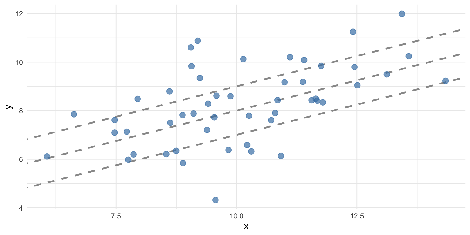

The best-fitting line (pt. 3)

We can also try the same intercept but different slopes.

# Create the plot
ggplot(df, aes(x = x, y = y)) +
  # Add several "possible" lines
  geom_abline(intercept = 3, slope = 0.75, color = "gray60", linetype = "dashed", linewidth = 1) +
  geom_abline(intercept = 3, slope = 0.5, color = "gray60", linetype = "dashed", linewidth = 1) +
  geom_abline(intercept = 3, slope = 0.25, color = "gray60", linetype = "dashed", linewidth = 1) +
  # Add data points
  geom_point(color = "steelblue", size = 3, alpha = 0.7) +
  theme_minimal()

Some lines are better than others

The line of best fit minimizes the residual error, i.e., the difference between the predictions (the line) and the actual values.

\(RSS = \sum_{i=1}^{N} (\hat{y_i} - y_i^2)\)

For each data point \(i\), subtract the actual value \(y_i\) from the predicted value \(\hat{y_i}\).
Then, square that difference.
Then, sum all those squared differences.

Tip

Intuition: A “better” line is one that has smaller differences between the predicted and actual values.

MSE: Mean-squared error

The mean-squared error (MSE) is the average squared error (as opposed to the sum).

Calculate \(RSS\).
Then, divide by \(N\).
Note that RMSE is the root of MSE.

Calculating MSE for a line

We can compare the MSE for two different lines for the same data.

y_pred1 = x * 1.5 + 2 ### Predictions from slope = 1.5 and intercept = 2
y_pred2 = x * .5 + 3 ### Predictions from slope = .5 and intercept = 3

mse_1 = sum((y_pred1 - y)**2)/length(y_pred1)
mse_2 = sum((y_pred2 - y)**2)/length(y_pred2)
print(mse_1)

[1] 83.65316

print(mse_2)

[1] 1.855965

Standard error of the estimate

The standard error of the estimate is a measure of the expected prediction error, i.e., how much your predictions are “wrong” on average.

\(S_{Y|X} = \sqrt{\frac{RSS}{n-2}}\)

How much, on average, do we expect \(\hat{Y}\) to deviate from \(Y\)?
A smaller number means a better fit.

Calculating standard error of the estimate

We can calculate standard error of the estimate:

sy_1 = sqrt(sum((y_pred1 - y)**2)/(length(y_pred1)-2))
sy_2 = sqrt(sum((y_pred2 - y)**2)/(length(y_pred2)-2))
print(sy_1)

[1] 9.334812

print(sy_2)

[1] 1.39043

Evaluating with R-squared

The \(R^2\), or coefficient of determination, measures the proportion of variance in \(Y\) explained by the model.

\(R^2 = 1 - \frac{RSS}{SS_Y}\)

Where \(SS_Y\) is the sum of squared error in \(Y\).

💭 Check-in

What does this formula mean and why does it measure the proportion of variance in \(Y\) explained by the model?

Decomposing \(R^2\)

\(R^2 = 1 - \frac{RSS}{SS_Y}\)

\(RSS\) refers to the unexplained (residual) variance in \(Y\) from the model.
\(SS_Y\) is the total variance in \(Y\) (i.e., before even fitting the model).
Thus, \(\frac{RSS}{SS_Y}\) captures the proportion of unexplained variance by the model.
- If \(\frac{RSS}{SS_Y} = 1\), the model has explained no variance.
- If \(\frac{RSS}{SS_Y} = 0\), the model has explained all variance.
And \(1 - \frac{RSS}{SS_Y}\) captures the proportion of explained variance.

Key assumptions of linear regression

Ordinary least squares (OLS) regression has a few key assumptions.

Assumption	What it means	Why it matters
Linearity	The relationship between \(X\) and \(Y\) is linear	OLS fits a straight line, so if the true relationship is curved, predictions will be systematically biased
Independence	The observations are independent of each other	Dependent observations (e.g., repeated measures, time series) violate the assumption that errors are uncorrelated, leading to underestimated standard errors and invalid p-values
Homoscedasticity	The variance of residuals is constant across all levels of \(X\) (equal spread)	If variance changes with \(X\) (heteroscedasticity), standard errors will be incorrect: some coefficients appear more/less significant than they truly are
Normality of residuals	The errors are approximately normally distributed	Needed for valid confidence intervals and hypothesis tests (p-values). Less critical with large samples due to the Central Limit Theorem.

Interim summary

In statistical modeling, we aim to construct models of our data.
Linear regression is a specific (high-bias) model.
The goal of linear regression is to identify the best-fitting line for our data, i.e., to reduce the residual sum of squares (RSS).
Linear regression rests on a few assumptions about the data (more on this in an upcoming lecture).

Part 3: Linear regression in R

Using and interpreting fit lm models, using broom.

The `lm` function

A linear model can be fit using the lm function.

Supply a formula (i.e., y ~ x).
Supply the data (i.e., a dataframe).
Usage: lm(data = df_name, y ~ x).
- Where y and x are columns in df_name.

Loading a dataset

To illustrate linear regression in R, we’ll work with a sample dataset.

df_income <- read_csv("https://raw.githubusercontent.com/seantrott/ucsd_css211_datasets/main/main/regression/income.csv")

Rows: 30 Columns: 3
── Column specification ────────────────────────────────────────────────────────
Delimiter: ","
dbl (3): Education, Seniority, Income

ℹ Use `spec()` to retrieve the full column specification for this data.
ℹ Specify the column types or set `show_col_types = FALSE` to quiet this message.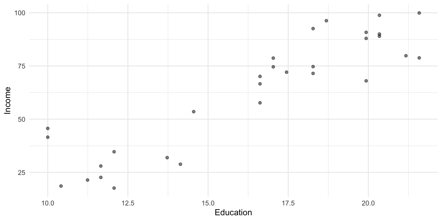

df_income %>%
  ggplot(aes(x = Education, y = Income)) +
  geom_point(alpha = .5) +
  theme_minimal()

Visualizing the model fit

As we discussed before, geom_smooth(method = "lm") can be used to plot a regression line over your data.

df_income %>%
  ggplot(aes(x = Education, y = Income)) +
  geom_point(alpha = .5) +
  geom_smooth(method = "lm", se = TRUE, color = "red") +
  theme_minimal()

`geom_smooth()` using formula = 'y ~ x'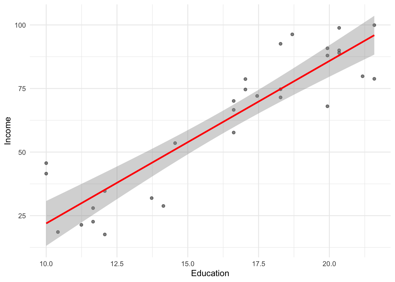

Tip

But to actually fit a model, we need to use lm.

Fitting an `lm` model

Calling summary on a fit lm model object returns information about the coefficients and the overall model fit.

mod = lm(data = df_income, Income ~ Education)
summary(mod)


Call:
lm(formula = Income ~ Education, data = df_income)

Residuals:
    Min      1Q  Median      3Q     Max 
-19.568  -8.012   1.474   5.754  23.701 

Coefficients:
            Estimate Std. Error t value Pr(>|t|)    
(Intercept) -41.9166     9.7689  -4.291 0.000192 ***
Education     6.3872     0.5812  10.990 1.15e-11 ***
---
Signif. codes:  0 '***' 0.001 '**' 0.01 '*' 0.05 '.' 0.1 ' ' 1

Residual standard error: 11.93 on 28 degrees of freedom
Multiple R-squared:  0.8118,    Adjusted R-squared:  0.8051 
F-statistic: 120.8 on 1 and 28 DF,  p-value: 1.151e-11

Understanding `summary` output

Calling summary returns information about the coefficients of our model, as well as indicators of model fit.

summ = summary(mod) 
summ$coefficients

              Estimate Std. Error   t value     Pr(>|t|)
(Intercept) -41.916612  9.7689490 -4.290801 1.918257e-04
Education     6.387161  0.5811716 10.990148 1.150567e-11

summ$r.squared

[1] 0.8118069

Estimate: fit intercept and slope coefficients.
Std. Error: estimated standard error for those coefficients.
t value: the t-statistic for those coefficients (slope / SE).
p-value: the probability of obtaining a t-statistic that large assuming the null hypothesis.
Multiple R-squared: proportion of variance in y explained by x.
Residual standard error: The standard error of the estimate.

Interpreting coefficients

There are a few relevant things to note about coefficients:

The estimate tells you the direction (sign) and degree (magnitude) of the relationship.
The p-value tells you whether a relationship of this size would be expected assuming there was no effect (i.e., the null hypothesis).
- More on this in an upcoming lecture!

💭 Check-in

How would you report and interpret the intercept and slope we obtained for Income ~ Education? (As a reminder, \(\beta_0 = -41.9\) and \(\beta_1 = 6.4\).)

The `broom` package

The broom package is also an easy way to quickly (and tidily) extract coefficient estimates.

df_coef = broom::tidy(mod)
df_coef

# A tibble: 2 × 5
  term        estimate std.error statistic  p.value
  <chr>          <dbl>     <dbl>     <dbl>    <dbl>
1 (Intercept)   -41.9      9.77      -4.29 1.92e- 4
2 Education       6.39     0.581     11.0  1.15e-11

Plotting coefficients

Once coefficients are in a dataframe, we can plot them using ggplot: a great way to visualize model fits!

df_coef %>%
  ggplot(aes(x = term, y = estimate)) +
  geom_point() +
  geom_errorbar(aes(x = term, y = estimate, 
                    ymin = estimate - std.error, 
                    ymax = estimate + std.error)) +
  coord_flip() +
  geom_hline(yintercept = 0, linetype = "dotted") +
  theme_minimal()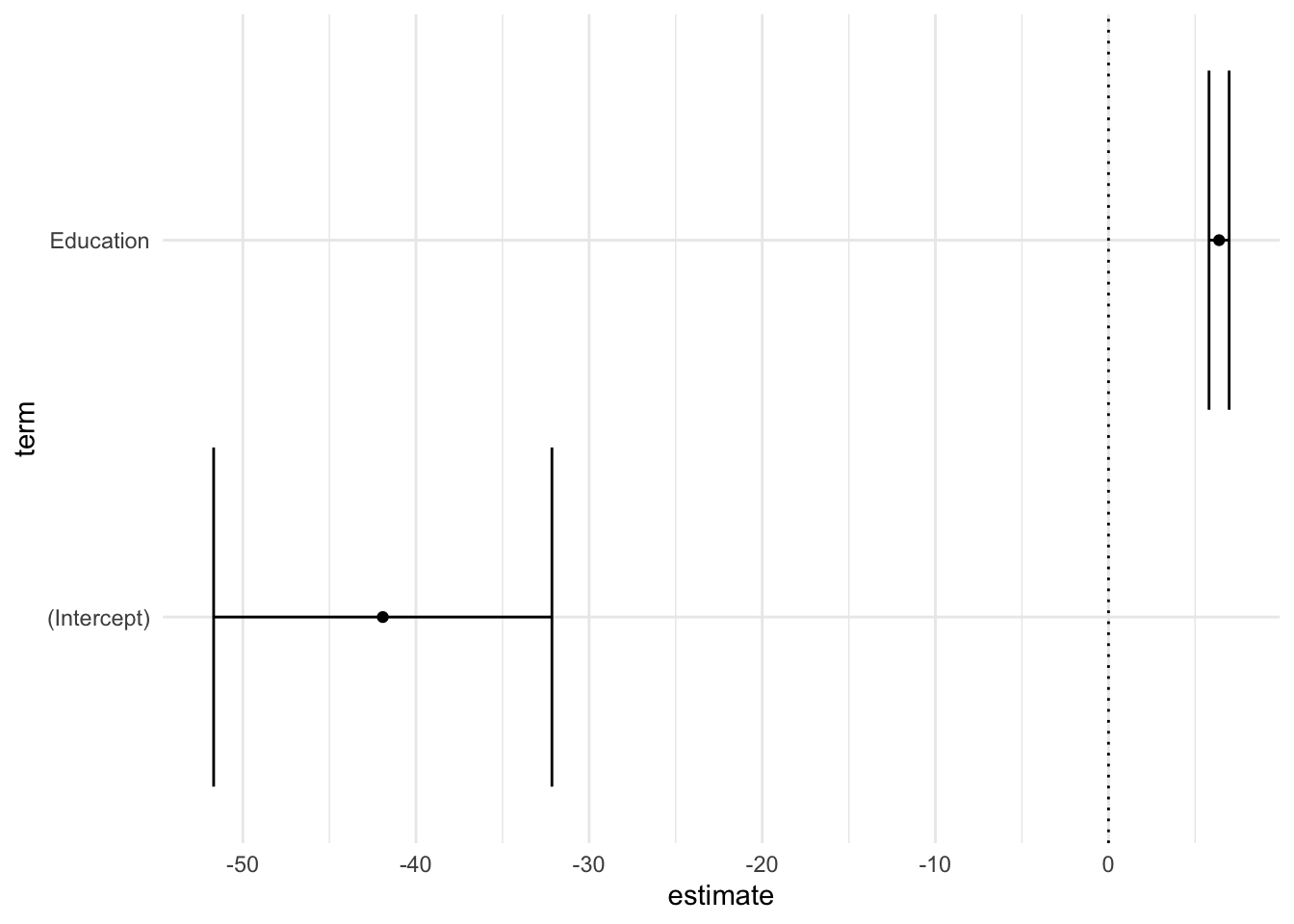

Overall model fit with `glance`

broom::glance() provides a tidy summary of overall model statistics.

broom::glance(mod)

# A tibble: 1 × 12
  r.squared adj.r.squared sigma statistic  p.value    df logLik   AIC   BIC
      <dbl>         <dbl> <dbl>     <dbl>    <dbl> <dbl>  <dbl> <dbl> <dbl>
1     0.812         0.805  11.9      121. 1.15e-11     1  -116.  238.  242.
# ℹ 3 more variables: deviance <dbl>, df.residual <int>, nobs <int>

r.squared: proportion of variance explained
adj.r.squared: adjusted for number of predictors
sigma: residual standard error
p.value: p-value for the F-statistic

Using `lm` with `%>%`

If you like the %>% syntax, you can integrate lm into a series of pipe operations.

df_income %>%
  ## fit model
  lm(Income ~ Education, data = .) %>%
  ## tidy into dataframe
  broom::tidy()

# A tibble: 2 × 5
  term        estimate std.error statistic  p.value
  <chr>          <dbl>     <dbl>     <dbl>    <dbl>
1 (Intercept)   -41.9      9.77      -4.29 1.92e- 4
2 Education       6.39     0.581     11.0  1.15e-11

Making predictions

Once we’ve fit a model, we can use it to make predictions for new data!

# Predict income for someone with 16 years of education
new_data <- data.frame(Education = 16)
predict(mod, newdata = new_data)

       1 
60.27797

# Or for multiple values
new_data <- data.frame(Education = c(12, 16, 20))
predict(mod, newdata = new_data, interval = "confidence")

       fit      lwr      upr
1 34.72932 27.86206 41.59659
2 60.27797 55.79413 64.76181
3 85.82661 79.62969 92.02353

Visualizing residuals

We can also assess the residuals.

df_income %>%
  mutate(resid = residuals(mod)) %>%
  ggplot(aes(x = Income, y = resid)) +
  geom_hline(yintercept = 0, linetype = "dashed", color = "red") +
  geom_point() +
  theme_minimal()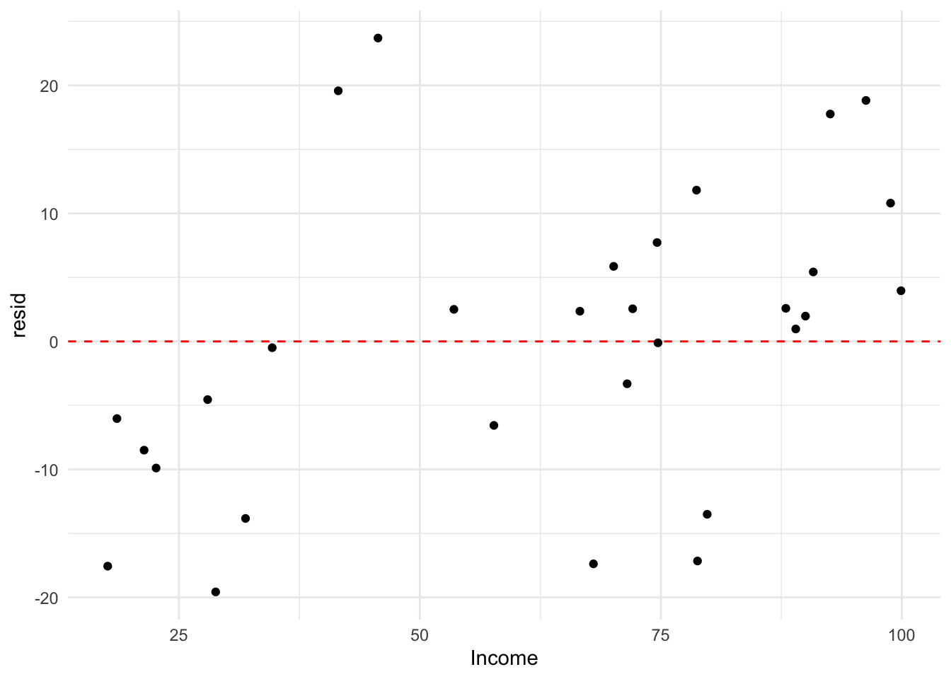

What about categorical predictors?

A categorical (or qualitative) variable takes on one of several discrete values.

df_stroop <- read_csv("https://raw.githubusercontent.com/seantrott/ucsd_css211_datasets/main/main/regression/stroop.csv")

Rows: 48 Columns: 2
── Column specification ────────────────────────────────────────────────────────
Delimiter: ","
chr (1): Condition
dbl (1): RT

ℹ Use `spec()` to retrieve the full column specification for this data.
ℹ Specify the column types or set `show_col_types = FALSE` to quiet this message.

head(df_stroop, 3)

# A tibble: 3 × 2
  Condition    RT
  <chr>     <dbl>
1 Congruent 12.1 
2 Congruent 16.8 
3 Congruent  9.56

💭 Check-in

How might you model and interpret the effect of a categorical variable?

Contrast coding

A common approach is to use the mean of one level (e.g., Congruent) as the intercept; the slope then represents the difference in means across those levels.

### Actual means
df_stroop %>%
  group_by(Condition) %>%
  summarise(mean_RT = mean(RT))

# A tibble: 2 × 2
  Condition   mean_RT
  <chr>         <dbl>
1 Congruent      14.1
2 Incongruent    22.0

### Fit coefficients
lm(data = df_stroop, RT ~ Condition)$coefficients

         (Intercept) ConditionIncongruent 
           14.051125             7.964792

Conclusion

Linear regression is a foundational tool in your modeling toolbox.
R simplifies fitting and interpreting regressions:
- lm: fit the model.
- summary/broom::tidy/broom::glance: interpret the model coefficients and \(R^2\).
- predict: get predictions from the model.
Next time, we’ll discuss advanced issues, like multiple predictors.

Goals of the lecture

Part 1: Modeling

From descriptions to models

Why models?

Models encode functions

Models aren’t perfect

Models have trade-offs

Part 2: Univariate linear regression

Linear regression: basics

The line of best fit

The best-fitting line (pt. 1)

The best-fitting line (pt. 2)

The best-fitting line (pt. 3)

Some lines are better than others

MSE: Mean-squared error

Calculating MSE for a line

Standard error of the estimate

Calculating standard error of the estimate

Evaluating with R-squared

Decomposing \(R^2\)

Key assumptions of linear regression

Interim summary

Part 3: Linear regression in R

The lm function

Loading a dataset

Visualizing the model fit

Fitting an lm model

Understanding summary output

Interpreting coefficients

The broom package

Plotting coefficients

Overall model fit with glance

Using lm with %>%

Making predictions

Visualizing residuals

What about categorical predictors?

Contrast coding

Conclusion

The `lm` function

Fitting an `lm` model

Understanding `summary` output

The `broom` package

Overall model fit with `glance`

Using `lm` with `%>%`