Goals of the lecture
Multiple regression : beyond single predictors.
Modeling interaction effects.
Advanced topics in regression:
Understanding standard errors and coefficient sampling distributions .
Heteroscedasticity.
Multicollinearity.
Part 1: Multiple regression
Multiple predictors, interpreting coefficients, and interaction effects.
What is multiple regression
Multiple regression means building a regression model (e.g., linear regression) with more than one predictor.
There are a few reasons to do this:
Multiple predictors helps “adjust for” multiple correlated effects, i.e., \(X_1\) and \(X_2\) .
Tells us the effect of \(X_1\) on \(Y\) , holding constant the effect of \(X_2\) on \(Y\) .
Important for addressing confounding variables .
In general, adding more predictors often results in more powerful models .
Better for predicting things in the real world!
Loading a dataset
Fortunately, we can still use lm to build multiple regression models in R. To get started, let’s load the income dataset we used in previous lecutres.
### Loading the tidyverse library (tidyverse)
── Attaching core tidyverse packages ──────────────────────── tidyverse 2.0.0 ──
✔ dplyr     1.1.4     ✔ readr     2.1.5
✔ forcats   1.0.0     ✔ stringr   1.5.1
✔ ggplot2   3.5.2     ✔ tibble    3.2.1
✔ lubridate 1.9.4     ✔ tidyr     1.3.1
✔ purrr     1.0.4
── Conflicts ────────────────────────────────────────── tidyverse_conflicts() ──
✖ dplyr::filter() masks stats::filter()
✖ dplyr::lag()    masks stats::lag()
ℹ Use the conflicted package (<http://conflicted.r-lib.org/>) to force all conflicts to become errors
<- read_csv ("https://raw.githubusercontent.com/seantrott/ucsd_css211_datasets/main/main/regression/income.csv" )
Rows: 30 Columns: 3
── Column specification ────────────────────────────────────────────────────────
Delimiter: ","
dbl (3): Education, Seniority, Income

ℹ Use `spec()` to retrieve the full column specification for this data.
ℹ Specify the column types or set `show_col_types = FALSE` to quiet this message.
Building a multiple regression model
To add multiple predictors to our formula, simply use the + syntax.
= lm (data = df_income,~ Seniority + Education)summary (mod_multiple)
Call:
lm(formula = Income ~ Seniority + Education, data = df_income)

Residuals:
   Min     1Q Median     3Q    Max
-9.113 -5.718 -1.095  3.134 17.235

Coefficients:
             Estimate Std. Error t value Pr(>|t|)
(Intercept) -50.08564    5.99878  -8.349 5.85e-09 ***
Seniority     0.17286    0.02442   7.079 1.30e-07 ***
Education     5.89556    0.35703  16.513 1.23e-15 ***
---
Signif. codes:  0 '***' 0.001 '**' 0.01 '*' 0.05 '.' 0.1 ' ' 1

Residual standard error: 7.187 on 27 degrees of freedom
Multiple R-squared:  0.9341,    Adjusted R-squared:  0.9292
F-statistic: 191.4 on 2 and 27 DF,  p-value: < 2.2e-16
Try building two models with each of those predictors on their own. Compare the coefficient values and \(R^2\) . Any differences?
Comparing coefficients to single predictors
In general, we see that the coefficients are pretty similar from the single-variable models and the multiple-variable models, though generally reduced in the multiple-variable model.
# Model 1: Single predictor - Seniority only <- lm (Income ~ Seniority, data = df_income)# Model 2: Single predictor - Education only <- lm (Income ~ Education, data = df_income)# Model 3: Multiple regression - Both predictors <- lm (Income ~ Seniority + Education, data = df_income)$ coefficients
(Intercept)   Seniority
  39.158326    0.251288
$ coefficients
(Intercept)   Education
 -41.916612    6.387161
$ coefficients
(Intercept)   Seniority   Education
-50.0856388   0.1728555   5.8955560
Comparing fit to single predictors
We also see that the model with multiple predictors achieves a better \(R^2\) .
summary (mod_seniority)$ r.squaredsummary (mod_education)$ r.squaredsummary (mod_multiple)$ r.squared
Are there any potential concerns with using standard \(R^2\) here?
Using adjusted R-squared
Adjusted \(R^2\) is a modified version of \(R^2\) that accounts for the fact that adding more variables will always slightly improve model fit .
\(R^2_{adj} = 1 - \frac{RSS/(n - p - 1)}{SS_Y/(n - 1)}\)
Where:
\(n\) : number of observations.\(p\) : number of parameters in model.
summary (mod_seniority)$ adj.r.squaredsummary (mod_education)$ adj.r.squaredsummary (mod_multiple)$ adj.r.squared
As \(p\) increases, the numerator decreases, i.e., it’s a penalty for adding more predictors.
AIC: Another metric of fit
Akaike Information Criterion (or AIC ) is another commonly used metric of model fit .
\(AIC = 2k - 2\ln(L)\)
Where:
\(k\) is the number of parameters.\(L\) is the likelihood of the data under the model (we’ll discuss this soon!).
Unlike \(R^2\) , a lower AIC is better. We’ll talk more about model likelihood later in the course!
Your turn: using mtcars
Now, let’s apply this using the mtcars dataset:
Try to predict mpg from wt. Interpret the coefficients and model fit.
Then try to predict mpg from am. Interpret the coefficients and model fit. Note that you might need to convert am into a factor first.
Finally, predict mpg from both variables. Interpret the coefficients and model fit.
Writing out the linear equation
It’s often helpful to practice writing out the linear equations for a fit lm. Let’s write out the equations for the multiple variable model above.
\(Y_{mpg} = 37.32 - 5.35X_{wt} - 0.02X_{am}\)
What about interactions between our terms?
Interaction effects
An interaction effect occurs when the effect of one variable (\(X_1\) ) depends on the value of another variable (\(X_2\) ).
So far, we’ve assumed variables have roughly additive effects .
An interaction removes that assumption.
In model, allows for \(X_1 * X_2\) , i.e., a multiplicative effect .
Examples of interaction effects
Any set of variables could interact (including more than two!), but it’s often easiest to interpret interactions with categorical variables .
Food x Condiment: The enjoyment of a Food (ice cream vs. hot dog) depends on the Condiment (Chocolate vs. Ketchup).Treatment x Gender: The effect of some treatment depends on the Gender of the recipient.Brain Region x Task: The activation in different Brain Regions depends on the Task (e.g., motor vs. visual).
Building an interaction effect
We can interpret the coefficients as follows:
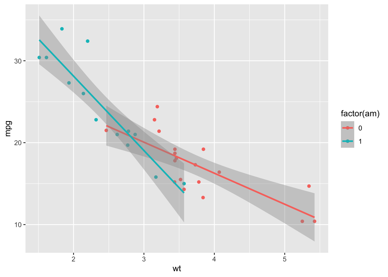
Intercept : Automatic cars (am = 0) with wt = 0 have expected mpg of 31.wt: As wt increases, we expect automatic cars to decrease mpg by about 3.7.factor(am): Holding wt constant, manual cars have an expected mpg of about 14 more than automatic cars.Interaction : Among manual cars , increases in wt correspond to even sharper declines in expected mpg.
= lm (data = mtcars, mpg ~ am * wt)summary (mod_int)
Call:
lm(formula = mpg ~ am * wt, data = mtcars)

Residuals:
    Min      1Q  Median      3Q     Max
-3.6004 -1.5446 -0.5325  0.9012  6.0909

Coefficients:
            Estimate Std. Error t value Pr(>|t|)
(Intercept)  31.4161     3.0201  10.402 4.00e-11 ***
am           14.8784     4.2640   3.489  0.00162 **
wt           -3.7859     0.7856  -4.819 4.55e-05 ***
am:wt        -5.2984     1.4447  -3.667  0.00102 **
---
Signif. codes:  0 '***' 0.001 '**' 0.01 '*' 0.05 '.' 0.1 ' ' 1

Residual standard error: 2.591 on 28 degrees of freedom
Multiple R-squared:  0.833, Adjusted R-squared:  0.8151
F-statistic: 46.57 on 3 and 28 DF,  p-value: 5.209e-11
Visualizing an interaction
By default, R will draw different regression lines for each level of a categorical factor we’ve added an aes for.
%>% ggplot (aes (x = wt, y = mpg, color = factor (am))) + geom_point () + geom_smooth (method = "lm" )
`geom_smooth()` using formula = 'y ~ x'
Interim summary
Multiple regression models are often more powerful than single-variable models.
In some cases, adding an interaction helps account for relationships that depend on another variable.
But adding multiple variables does make interpretation slightly more challenging.
Part 2: Advanced topics
Standard errors, heteroscedasticity, and multicollinearity.
Coefficient standard errors (SEs)
The standard error of a coefficient measures the uncertainty in the estimated coefficient value.
When we inspect the output of a fit lm model, we can see not only the coefficients but the standard errors (Std. Error):
Call:
lm(formula = Income ~ Education, data = df_income)

Residuals:
    Min      1Q  Median      3Q     Max
-19.568  -8.012   1.474   5.754  23.701

Coefficients:
            Estimate Std. Error t value Pr(>|t|)
(Intercept) -41.9166     9.7689  -4.291 0.000192 ***
Education     6.3872     0.5812  10.990 1.15e-11 ***
---
Signif. codes:  0 '***' 0.001 '**' 0.01 '*' 0.05 '.' 0.1 ' ' 1

Residual standard error: 11.93 on 28 degrees of freedom
Multiple R-squared:  0.8118,    Adjusted R-squared:  0.8051
F-statistic: 120.8 on 1 and 28 DF,  p-value: 1.151e-11
Does a larger SE correspond to more or less uncertainty about our estimate?
The sampling distribution of coefficients
If we could repeatedly sample from our population and fit our model each time, we’d get a distribution of coefficient estimates .
This is called the sampling distribution of the coefficient.
The standard error is the standard deviation of this sampling distribution.
It tells us: “If we repeated this study many times, how much would our coefficient estimate vary?”
Which properties affect the standard deviation of that sampling distribution?
Calculating the SE
For a simple linear regression, the SE of the slope coefficient is:
\(SE(\beta_1) = \sqrt{\frac{\sum(y_i - \hat{y}_i)^2}{(n-2)\sum(x_i - \bar{x})^2}}\)
Numerator : Larger residuals → more uncertainty → larger SEDenominator : More data points and more spread in \(X\) → less uncertainty → smaller SEFor multiple regression, the calculation is more complex (involves matrix algebra)
Fortunately, R calculates this for us!
You will not be expected to calculate this from scratch!
The t-statistic
The t-statistic measures how many standard errors a coefficient is away from zero.
\(t = \frac{\hat{\beta} - 0}{SE(\hat{\beta})}\)
# Extract coefficient and SE for Education <- summary (mod_education)$ coefficients["Education" , "Estimate" ]<- summary (mod_education)$ coefficients["Education" , "Std. Error" ]# Calculate t-statistic manually <- coef_value / se_value
This matches the t value column in our summary output!
Interpreting the t-statistic
The t-statistic follows a t-distribution under the null hypothesis that \(\beta = 0\) .
Rule of thumb : \(|t| \geq 2\) typically indicates statistical significance (p < 0.05).More precisely: We calculate the probability of observing a \(|t|\) this large (or larger) if the true coefficient were zero.
This probability is the p-value .
Looking at our mod_education output, is the Education coefficient significantly different from zero?
Confidence intervals
We can use the SE to construct confidence intervals around our coefficient estimates:
\(\hat{\beta} \pm t_{critical} \times SE(\hat{\beta})\)
# 95% confidence intervals for our regression model confint (mod_education)
                 2.5 %     97.5 %
(Intercept) -61.927397 -21.905827
Education     5.196685   7.577637
Your turn: SEs and t-statistics
Using your mtcars model from earlier predicting mpg from wt and am:
Which coefficient has the largest standard error?
Which coefficient has the smallest p-value (most significant)?
Calculate 99% confidence intervals using confint(model, level = 0.99).
Heteroscedasticity
Heteroscedasticity occurs when the variance of residuals is not constant across all levels of the predictors.
Homoscedasticity (the ideal): Residuals have constant variance.Heteroscedasticity (a problem): Residual variance changes with predictor values.This violates one of the key assumptions of linear regression!
Consequences: Standard errors become unreliable, affecting our hypothesis tests.
Why would heteroscecasticity affect our interpretation of standard errors?
Heteroscedasticity and prediction error
The standard error of the estimate gives us an estimate of how much prediction error to expect.
With homoscedasticity, our expected error shouldn’t really depend on \(X\) .
But with heteroscedasticity, our margin of error might actually vary as a function of \(X\) .
Yet we only have a single estimate of our prediction error, which might overestimate or underestimate error for a given \(X\) value.
Why heteroscedasticity biases SEs
The key insight:
OLS gives equal weight to all observations when estimating SEs.
But with heteroscedasticity, some observations have more noise than others.
High-variance observations should be trusted less , but OLS doesn’t know this.
Result: SEs don’t accurately reflect true uncertainty.
Detecting heteroscedasticity
We can diagnose heteroscedasticity by plotting residuals vs. fitted values:
# Create diagnostic plot tibble (fitted = fitted (mod_multiple),residuals = residuals (mod_multiple)%>% ggplot (aes (x = fitted, y = residuals)) + geom_point (alpha = 0.5 ) + geom_hline (yintercept = 0 , linetype = "dashed" , color = "red" ) + labs (title = "Residuals vs. Fitted Values" ,x = "Fitted Values" , y = "Residuals" ) + theme_minimal ()
Look for: funnel shapes, increasing/decreasing spread, or other patterns.
What to do about heteroscedasticity?
Several options to address heteroscedasticity:
We won’t be covering (2) or (3), but there are R packages for implementing both.
Multicollinearity
Multicollinearity occurs when predictor variables are highly correlated with each other.
Makes it difficult to isolate the individual effect of each predictor.
Leads to unstable coefficient estimates with large standard errors.
Coefficients may have unexpected signs or magnitudes.
Does NOT affect predictions, but makes interpretation problematic.
Multicollinearity: The core problem
When predictors are highly correlated, the model struggles to determine which predictor is “responsible” for variation in Y.
Consider predicting income from: - Years of education - Number of graduate degrees
These are highly correlated - more years usually means more degrees.
The model faces a credit assignment challenge : Is income higher because of years OR degrees?
Many combinations of coefficients can fit the data equally well.
Result: Coefficients become unstable and uncertain .
Example: Detecting multicollinearity
Let’s check the correlation between our predictors:
# Correlation between predictors cor (df_income$ Seniority, df_income$ Education)# Visualize the relationship %>% ggplot (aes (x = Seniority, y = Education)) + geom_point (alpha = 0.5 ) + geom_smooth (method = "lm" ) + labs (title = "Relationship between Seniority and Education" ) + theme_minimal ()
`geom_smooth()` using formula = 'y ~ x'
Variance Inflation Factor (VIF)
The VIF quantifies how much the variance of a coefficient is inflated due to multicollinearity.
Loading required package: carData
The following object is masked from 'package:dplyr':

    recode
The following object is masked from 'package:purrr':

    some
Seniority Education
 1.039324  1.039324
VIF = 1 : No correlation with other predictorsVIF < 5 : Generally acceptableVIF > 10 : Serious multicollinearity problemVIF > 5 : Some concern, investigate further
Understanding VIF: The concept
VIF (Variance Inflation Factor) quantifies how much multicollinearity inflates the variance of a coefficient.
From the formula on the previous slide:
\(VIF_j = \frac{1}{1-R^2_j}\)
Where \(R^2_j\) is the R-squared from regressing predictor \(X_j\) on all other predictors.
Interpretation : “How much is the variance of \(\hat{\beta}_j\) inflated compared to if \(X_j\) were uncorrelated with other predictors?”If \(X_j\) is uncorrelated with others: \(R^2_j = 0\) → \(VIF = 1\) (no inflation)
If \(X_j\) is highly correlated with others: \(R^2_j\) close to 1 → \(VIF\) is large
What to do about multicollinearity?
Several strategies to address multicollinearity:
Remove one of the correlated predictorsCombine correlated predictors (e.g., create an index)Use principal components analysis (PCA) to create uncorrelated predictors
Use regularization methods (Ridge, Lasso regression)
Collect more data with greater variation in predictors
The best solution depends on your research question and theoretical considerations!
Your turn: Diagnostics
Using the mtcars dataset:
Build a model predicting mpg from wt, hp, and disp
Check for multicollinearity using cor() and vif()
Create a residual plot to check for heteroscedasticity
What potential issues do you notice?
Final summary
Standard errors quantify uncertainty in coefficient estimatest-statistics test whether coefficients differ significantly from zeroHeteroscedasticity (non-constant variance) violates regression assumptionsMulticollinearity (correlated predictors) inflates standard errors and makes interpretation difficultBoth issues can be diagnosed and addressed with appropriate techniques
Always check your model assumptions!
Key takeaways
Multiple regression allows us to model complex relationships
Adding interactions captures when one variable’s effect depends on another
Adjusted \(R^2\) and AIC help compare models with different numbers of predictorsUnderstanding SEs helps us assess the reliability of our estimates
Checking assumptions (homoscedasticity, no multicollinearity) is crucial
When assumptions are violated, specialized techniques can help